gretton12a.dvi

Journal of Machine Learning Research 13 (2012) 723-773 Submitted 4/08; Revised 11/11; Published 3/12

A Kernel Two-Sample Test

Arthur Gretton

∗

ARTHUR.GRETTON@GMAIL.COM

MPI for Intelligent Systems

Spemannstrasse 38

72076 T

ubingen, Germany

Karsten M. Borgwardt

†

KARSTEN.BORGWARDT@TUEBINGEN.MPG.DE

Machine Learning and Computational Biology Research Group

Max Planck Institutes T

ubingen

Spemannstrasse 38

72076 T

ubingen, Germany

Malte J. Rasch

‡

MALTE@MAIL.BNU.EDU.CN

19 XinJieKouWai St.

State Key Laboratory of Cognitive Neuroscience and Learning,

Beijing Normal University,

Beijing, 100875, P.R. China

Bernhard Sch

olkopf BERNHARD.SCHOELKOPF@TUEBINGEN.MPG.DE

MPI for Intelligent Systems

Spemannstrasse 38

72076, T

ubingen, Germany

Alexander Smola

ALEX@SMOLA.ORG

Yahoo! Research

2821 Mission College Blvd

Santa Clara, CA 95054, USA

Editor: Nicolas Vayatis

Abstract

We propose a framework for analyzing and comparing distributions, which we use to construct sta-

tistical tests to determine if two samples are drawn from different distributions. Our test statistic is

the largest difference in expectations over functions in the unit ball of a reproducing kernel Hilbert

space (RKHS), and is called the maximum mean discrepancy (MMD). We present two distribution-

free tests based on large deviation bounds for the MMD, and a third test based on the asymptotic

distribution of this statistic. The MMD can be computed in quadratic time, although efﬁcient linear

time approximations are available. Our statistic is an instance of an integral probability metric, and

various classical metrics on distributions are obtained when alternative function classes are used

in place of an RKHS. We apply our two-sample tests to a variety of problems, including attribute

matching for databases using the Hungarian marriage method, where they perform strongly. Ex-

cellent performance is also obtained when comparing distributions over graphs, for which these are

the ﬁrst such tests.

∗. Also at Gatsby Computational Neuroscience Unit, CSML, 17 Queen Square, London WC1N 3AR, UK.

†. This work was carried out while K.M.B. was with the Ludwig-Maximilians-Universit

at M

unchen.

‡. This work was carried out while M.J.R. was with the Graz University of Technology.

§. Also at The Australian National University, Canberra, ACT 0200, Australia.

2012 Arthur Gretton, Karsten M. Borgwardt, Malte J. Rasch, Bernhard Sch

olkopf and Alexander Smola.

GRETTON, BORGWARDT, RASCH, SCH

OLKOPF AND SMOLA

Keywords: kernel methods, two-sample test, uniform convergence bounds, schema matching,

integral probability metric, hypothesis testing

1. Introduction

We address the problem of comparing samples from two probability distributions, by proposing

statistical tests of the null hypothesis that these distributions are equal against the alternative hy-

pothesis that these distributions are different (this is called the two-sample problem). Such tests

have application in a variety of areas. In bioinformatics, it is of interest to compare microarray

data from identical tissue types as measured by different laboratories, to detect whether the data

may be analysed jointly, or whether differences in experimental procedure have caused systematic

differences in the data distributions. Equally of interest are comparisons between microarray data

from different tissue types, either to determine whether two subtypes of cancer may be treated as

statistically indistinguishable from a diagnosis perspective, or to detect differences in healthy and

cancerous tissue. In database attribute matching, it is desirable to merge databases containing mul-

tiple ﬁelds, where it is not known in advance which ﬁelds correspond: the ﬁelds are matched by

maximising the similarity in the distributions of their entries.

We test whether distributions p and q are different on the basis of samples drawn from each of

them, by ﬁnding a well behaved (e.g., smooth) function which is large on the points drawn from p,

and small (as negative as possible) on the points from q. We use as our test statistic the difference

between the mean function values on the two samples; when this is large, the samples are likely

from different distributions. We call this test statistic the Maximum Mean Discrepancy (MMD).

Clearly the quality of the MMD as a statistic depends on the class F of smooth functions that

deﬁne it. On one hand, F must be “rich enough” so that the population MMD vanishes if and only

if p = q. On the other hand, for the test to be consistent in power, F needs to be “restrictive” enough

for the empirical estimate of the MMD to converge quickly to its expectation as the sample size

increases. We will use the unit balls in characteristic reproducing kernel Hilbert spaces (Fukumizu

et al., 2008; Sriperumbudur et al., 2010b) as our function classes, since these will be shown to satisfy

both of the foregoing properties. We also review classical metrics on distributions, namely the

Kolmogorov-Smirnov and Earth-Mover’s distances, which are based on different function classes;

collectively these are known as integral probability metrics (M

uller, 1997). On a more practical

note, the MMD has a reasonable computational cost, when compared with other two-sample tests:

given m points sampled from p and n from q, the cost is O(m + n)

time. We also propose a test

statistic with a computational cost of O(m+n): the associated test can achieve a given Type II error

at a lower overall computational cost than the quadratic-cost test, by looking at a larger volume of

data.

We deﬁne three nonparametric statistical tests based on the MMD. The ﬁrst two tests are

distribution-free, meaning they make no assumptions regarding p and q, albeit at the expense of

being conservative in detecting differences between the distributions. The third test is based on the

asymptotic distribution of the MMD, and is in practice more sensitive to differences in distribution at

small sample sizes. The present work synthesizes and expands on results of Gretton et al. (2007a,b)

and Smola et al. (2007),

who in turn build on the earlier work of Borgwardt et al. (2006). Note that

1. In particular, most of the proofs here were not provided by Gretton et al. (2007a), but in an accompanying technical

report (Gretton et al., 2008a), which this document replaces.

724

A KERNEL TWO-SAMPLE TEST

the latter addresses only the third kind of test, and that the approach of Gretton et al. (2007a,b) is

rigorous in its treatment of the asymptotic distribution of the test statistic under the null hypothesis.

We begin our presentation in Section 2 with a formal deﬁnition of the MMD. We review the

notion of a characteristic RKHS, and establish that when F is a unit ball in a characteristic RKHS,

then the population MMD is zero if and only if p = q. We further show that universal RKHSs in

the sense of Steinwart (2001) are characteristic. In Section 3, we give an overview of hypothesis

testing as it applies to the two-sample problem, and review alternative test statistics, including the

distance between kernel density estimates (Anderson et al., 1994), which is the prior approach

closest to our work. We present our ﬁrst two hypothesis tests in Section 4, based on two different

bounds on the deviation between the population and empirical MMD. We take a different approach

in Section 5, where we use the asymptotic distribution of the empirical MMD estimate as the basis

for a third test. When large volumes of data are available, the cost of computing the MMD (quadratic

in the sample size) may be excessive: we therefore propose in Section 6 a modiﬁed version of the

MMD statistic that has a linear cost in the number of samples, and an associated asymptotic test.

In Section 7, we provide an overview of methods related to the MMD in the statistics and machine

learning literature. We also review alternative function classes for which the MMD deﬁnes a metric

on probability distributions. Finally, in Section 8, we demonstrate the performance of MMD-based

two-sample tests on problems from neuroscience, bioinformatics, and attribute matching using the

Hungarian marriage method. Our approach performs well on high dimensional data with low sample

size; in addition, we are able to successfully distinguish distributions on graph data, for which ours

is the ﬁrst proposed test.

A Matlab implementation of the tests is at www.gatsby.ucl.ac.uk/ ∼ gretton/mmd/mmd.htm.

2. The Maximum Mean Discrepancy

In this section, we present the maximum mean discrepancy (MMD), and describe conditions under

which it is a metric on the space of probability distributions. The MMD is deﬁned in terms of

particular function spaces that witness the difference in distributions: we therefore begin in Section

2.1 by introducing the MMD for an arbitrary function space. In Section 2.2, we compute both the

population MMD and two empirical estimates when the associated function space is a reproducing

kernel Hilbert space, and in Section 2.3 we derive the RKHS function that witnesses the MMD for

a given pair of distributions.

2.1 Deﬁnition of the Maximum Mean Discrepancy

Our goal is to formulate a statistical test that answers the following question:

Problem 1 Let x and y be random variables deﬁned on a topological space X, with respective

Borel probability measures p and q . Given observations X :=

{

,.. .,x

}

and Y :=

{

,.. .,y

}

independently and identically distributed (i.i.d.) from p and q, respectively, can we decide whether

p 6= q?

Where there is no ambiguity, we use the shorthand notation E

[ f(x)] := E

x∼p

[ f(x)] and E

[ f(y)] :=

y∼q

[ f(y)] to denote expectations with respect to p and q, respectively, where x ∼ p indicates x has

distribution p. To start with, we wish to determine a criterion that, in the population setting, takes

on a unique and distinctive value only when p = q. It will be deﬁned based on Lemma 9.3.2 of

Dudley (2002).

725

GRETTON, BORGWARDT, RASCH, SCH

OLKOPF AND SMOLA

Lemma 1 Let (X,d) be a metric space, and let p,q be two Borel probability measures deﬁned on

X. Then p = q if and only if E

( f(x)) = E

( f(y)) for all f ∈ C(X), where C(X) is the space of

bounded continuous functions on X.

AlthoughC(X) in principle allows us to identify p = q uniquely, it is not practical to work with such

a rich function class in the ﬁnite sample setting. We thus deﬁne a more general class of statistic, for

as yet unspeciﬁed function classes F, to measure the disparity between p and q (Fortet and Mourier,

1953; M

uller, 1997).

Deﬁnition 2 Let F be a class of functions f : X → R and let p, q,x,y, X,Y be deﬁned as above. We

deﬁne the maximum mean discrepancy (MMD) as

MMD[F, p,q] := sup

f∈F

[ f(x)] −E

[ f(y)]). (1)

In the statistics literature, this is known as an integral probability metric (M

uller, 1997). A biased

empirical estimate of the MMD is obtained by replacing the population expectations with empirical

expectations computed on the samples X and Y,

MMD

[F,X,Y] := sup

f∈F

∑

i=1

f(x

) −

∑

i=1

f(y

)

. (2)

We must therefore identify a function class that is rich enough to uniquely identify whether p = q,

yet restrictive enough to provide useful ﬁnite sample estimates (the latter property will be established

in subsequent sections).

2.2 The MMD in Reproducing Kernel Hilbert Spaces

In the present section, we propose as our MMD function class F the unit ball in a reproducing kernel

Hilbert space H. We will provide ﬁnite sample estimates of this quantity (both biased and unbiased),

and establish conditions under which the MMD can be used to distinguish between probability

measures. Other possible function classes F are discussed in Sections 7.1 and 7.2.

We ﬁrst review some properties of H (Sch

olkopf and Smola, 2002). Since H is an RKHS, the

operator of evaluation δ

mapping f ∈ H to f(x) ∈ R is continuous. Thus, by the Riesz represen-

tation theorem (Reed and Simon, 1980, Theorem II.4), there is a feature mapping φ(x) from X to

R such that f (x) =

f,φ(x)

. This feature mapping takes the canonical form φ(x) = k(x, ·) (Stein-

wart and Christmann, 2008, Lemma 4.19), where k(x

) : X ×X → R is positive deﬁnite, and

the notation k(x,·) indicates the kernel has one argument ﬁxed at x, and the second free. Note in

particular that

φ(x),φ(y)

= k(x, y). We will generally use the more concise notation φ(x) for the

feature mapping, although in some cases it will be clearer to write k(x, ·).

We next extend the notion of feature map to the embedding of a probability distribution: we

will deﬁne an element µ

∈ H such that E

f =

f,µ

for all f ∈ H, which we call the mean

embedding of p. Embeddings of probability measures into reproducing kernel Hilbert spaces are

well established in the statistics literature: see Berlinet and Thomas-Agnan (2004, Chapter 4) for

further detail and references. We begin by establishing conditions under which the mean embedding

exists (Fukumizu et al., 2004, p. 93), (Sriperumbudur et al., 2010b, Theorem 1).

2. The empirical MMD deﬁned below has an upward bias—we will deﬁne an unbiased statistic in the following section.

726

A KERNEL TWO-SAMPLE TEST

Lemma 3 If k(·,·) is measurable and E

k(x, x) < ∞ then µ

∈ H.

Proof The linear operator T

f := E

f for all f ∈ F is bounded under the assumption, since

≤ E

= E

f,φ(x)

≤ E



k(x, x)



Hence by the Riesz representer theorem, there exists a µ

∈ H such that T

f =

f,µ

. If we set

f = φ(t) = k(t,·), we obtain µ

(t) =

,k(t,·)

= E

k(t, x): in other words, the mean embedding

of the distribution p is the expectation under p of the canonical feature map.

We next show that the MMD may be expressed as the distance in H between mean embeddings

(Borgwardt et al., 2006).

Lemma 4 Assume the condition in Lemma 3 for the existence of the mean embeddings µ

, µ

satisﬁed. Then

MMD

[F, p, q] =



−µ



Proof

MMD

[F, p, q] =

sup

≤1

[ f(x)] −E

[ f(y)])

sup

≤1



−µ

, f





−µ



We now establish a condition on the RKHS H under which the mean embedding µ

is injective,

which indicates that MMD[F, p, q] = 0 is a metric

on the Borel probability measures on X. Evi-

dently, this property will not hold for all H: for instance, a polynomial RKHS of degree two cannot

distinguish between distributions with the same mean and variance, but different kurtosis (Sriperum-

budur et al., 2010b, Example 3). The MMD is a metric, however, when H is a universal RKHSs,

deﬁned on a compact metric space X. Universality requires that k(·,·) be continuous, and H be

dense in C(X) with respect to the L

∞

norm. Steinwart (2001) proves that the Gaussian and Laplace

RKHSs are universal.

Theorem 5 Let F be a unit ball in a universal RKHS H, deﬁned on the compact metric space X,

with associated continuous kernel k(·,·). Then MMD[F, p, q] = 0 if and only if p = q.

Proof The proof follows Cortes et al. (2008, Supplementary Appendix), whose approach is clearer

than the original proof of Gretton et al. (2008a, p. 4).

First, it is clear that p = q implies

3. According to Dudley (2002, p. 26) a metric d(x,y) satisﬁes the following four properties: symmetry, triangle in-

equality, d(x,x) = 0, and d(x, y) = 0 =⇒ x = y. A pseudo-metric only satisﬁes the ﬁrst three properties.

4. Note that the proof of Cortes et al. (2008) requires an application the of dominated convergence theorem, rather than

using the Riesz representation theorem to show the existence of the mean embeddings µ

and µ

as we did in Lemma

727

GRETTON, BORGWARDT, RASCH, SCH

OLKOPF AND SMOLA

MMD

{

F, p, q

}

is zero. We now prove the converse. By the universality of H, for any given ε > 0

and f ∈C(X) there exists a g ∈ H such that

f −g

∞

≤ ε.

We next make the expansion

f(x) −E

( f(y))

≤

f(x) −E

g(x)

g(x) −E

g(y)

g(y) −E

f(y)

The ﬁrst and third terms satisfy

f(x) −E

g(x)

≤ E

f(x) −g(x)

≤ ε.

Next, write

g(x) −E

g(y) =



g,µ

−µ



= 0,

since MMD

{

F, p, q

}

= 0 implies µ

= µ

. Hence

f(x) −E

( f(y))

≤ 2ε

for all f ∈C(X) and ε > 0, which implies p = q by Lemma 1.

While our result establishes the mapping µ

is injective for universal kernels on compact domains,

this result can also be shown in more general cases. Fukumizu et al. (2008) introduces the notion

of characteristic kernels, these being kernels for which the mean map is injective. Fukumizu et al.

establish that Gaussian and Laplace kernels are characteristic on R

, and thus that the associated

MMD is a metric on distributions for this domain. Sriperumbudur et al. (2008, 2010b) and Sripe-

rumbudur et al. (2011a) further explore the properties of characteristic kernels, providing a simple

condition to determine whether translation invariant kernels are characteristic, and investigating the

relation between universal and characteristic kernels on non-compact domains.

Given we are in an RKHS, we may easily obtain of the squared MMD,



−µ



, in terms of

kernel functions, and a corresponding unbiased ﬁnite sample estimate.

Lemma 6 Given x and x

′

independent random variables with distribution p, and y and y

′

indepen-

dent random variables with distribution q, the squared population MMD is

MMD

[F, p, q] = E

x,x

′



k(x, x

′

)



−2E

x,y

[k(x, y)]+ E

y,y

′



k(y, y

′

)



where x

′

is an independent copy of x with the same distribution, and y

′

is an independent copy of y.

An unbiased empirical estimate is a sum of two U-statistics and a sample average,

MMD

[F,X,Y] =

m(m−1)

∑

i=1

∑

j6=i

k(x

) +

n(n−1)

∑

i=1

∑

j6=i

k(y

)

−

∑

i=1

∑

j=1

k(x

). (3)

When m = n, a slightly simpler empirical estimate may be used. Let Z := (z

,.. .,z

) be m i.i.d.

random variables, where z := (x,y) ∼ p×q (i.e., x and y are independent). An unbiased estimate of

MMD

[F,X,Y] =

(m)(m−1)

∑

i6= j

h(z

), (4)

728

A KERNEL TWO-SAMPLE TEST

which is a one-sample U-statistic with

h(z

) := k(x

) + k(y

) −k(x

Proof Starting from the expression for MMD

[F, p, q] in Lemma 4,

MMD

[F, p, q] =



−µ



,µ



,µ



−2



,µ



= E

x,x

′



φ(x),φ(x

′

)



+ E

y,y

′



φ(y),φ(y

′

)



−2E

x,y

φ(x),φ(y)

The proof is completed by applying

φ(x),φ(x

′

)

= k(x, x

′

); the empirical estimates follow straight-

forwardly, by replacing the population expectations with their corresponding U-statistics and sample

averages. This statistic is unbiased following Serﬂing (1980, Chapter 5).

Note that MMD

may be negative, since it is an unbiased estimator of (MMD[F, p, q])

. The only

terms missing to ensure nonnegativity, however, are h(z

), which were removed to remove spuri-

ous correlations between observations. Consequently we have the bound

MMD

m(m−1)

∑

i=1

k(x

) + k(y

) −2k(x

) ≥ 0.

Moreover, while the empirical statistic for m = n is an unbiased estimate of MMD

, it does not have

minimum variance, since we ignore the cross-terms k(x

), of which there are O(n). From (3),

however, we see the minimum variance estimate is almost identical (Serﬂing, 1980, Section 5.1.4).

The biased statistic in (2) may also be easily computed following the above reasoning. Substi-

tuting the empirical estimates µ

∑

i=1

φ(x

) and µ

∑

i=1

φ(y

) of the feature space means

based on respective samples X and Y, we obtain

MMD

[F,X,Y] =

∑

i, j=1

k(x

) −

m,n

∑

i, j=1

k(x

) +

∑

i, j=1

k(y

)

. (5)

Note that the U-statistics of (3) have been replaced by V-statistics. Intuitively we expect the empir-

ical test statistic MMD[F,X,Y], whether biased or unbiased, to be small if p = q, and large if the

distributions are far apart. It costs O((m+ n)

) time to compute both statistics.

2.3 Witness Function of the MMD for RKHSs

We deﬁne the witness function f

∗

to be the RKHS function attaining the supremum in (1), and

its empirical estimate

∗

to be the function attaining the supremum in (2). From the reasoning in

Lemma 4, it is clear that

∗

(t) ∝



φ(t),µ

−µ



= E

[k(x,t)] −E

[k(y,t)],

∗

(t) ∝

φ(t),µ

−µ

∑

i=1

k(x

,t) −

∑

i=1

k(y

,t).

where we have deﬁned µ

= m

−1

∑

i=1

φ(x

), and µ

by analogy. The result follows since the unit

vector v maximizing

v, x

in a Hilbert space is v = x/

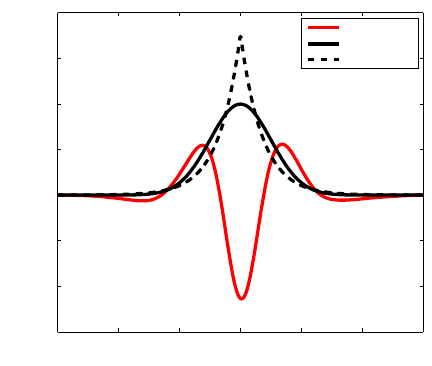
We illustrate the behavior of MMD in Figure 1 using a one-dimensional example. The data X

and Y were generated from distributions p and q with equal means and variances, with p Gaussian

729

GRETTON, BORGWARDT, RASCH, SCH

OLKOPF AND SMOLA

−6 −4 −2 0 2 4 6

−0.6

−0.4

−0.2

0.2

0.4

0.6

0.8

Prob. densities and

∗

(t)

∗

p (Gau ss)

q (L aplace)

Figure 1: Illustration of the function maximizing the mean discrepancy in the case where a Gaussian

is being compared with a Laplace distribution. Both distributions have zero mean and unit

variance. The function

∗

that witnesses the MMD has been scaled for plotting purposes,

and was computed empirically on the basis of 2×10

samples, using a Gaussian kernel

with σ = 0.5.

and q Laplacian. We chose F to be the unit ball in a Gaussian RKHS. The empirical estimate

∗

of the function f

∗

that witnesses the MMD—in other words, the function maximizing the mean

discrepancy in (1)—is smooth, negative where the Laplace density exceeds the Gaussian density (at

the center and tails), and positive where the Gaussian density is larger. The magnitude of

∗

is a

direct reﬂection of the amount by which one density exceeds the other, insofar as the smoothness

constraint permits it.

3. Background Material

We now present three background results. First, we introduce the terminology used in statistical

hypothesis testing. Second, we demonstrate via an example that even for tests which have asymp-

totically no error, we cannot guarantee performance at any ﬁxed sample size without making as-

sumptions about the distributions. Third, we review some alternative statistics used in comparing

distributions, and the associated two-sample tests (see also Section 7 for an overview of additional

integral probability metrics).

3.1 Statistical Hypothesis Testing

Having described a metric on probability distributions (the MMD) based on distances between their

Hilbert space embeddings, and empirical estimates (biased and unbiased) of this metric, we address

the problem of determining whether the empirical MMD shows a statistically signiﬁcant difference

between distributions. To this end, we brieﬂy describe the framework of statistical hypothesis testing

as it applies in the present context, following Casella and Berger (2002, Chapter 8). Given i.i.d.

730

A KERNEL TWO-SAMPLE TEST

samples X ∼ p of size m and Y ∼q of size n, the statistical test, T(X,Y) : X

×X

7→{0,1} is used

to distinguish between the null hypothesis H

: p = q and the alternative hypothesis H

: p 6= q.

This is achieved by comparing the test statistic

MMD[F,X,Y] with a particular threshold: if the

threshold is exceeded, then the test rejects the null hypothesis (bearing in mind that a zero population

MMD indicates p = q). The acceptance region of the test is thus deﬁned as the set of real numbers

below the threshold. Since the test is based on ﬁnite samples, it is possible that an incorrect answer

will be returned. A Type I error is made when p = q is rejected based on the observed samples,

despite the null hypothesis having generated the data. Conversely, a Type II error occurs when

p = q is accepted despite the underlying distributions being different. The level α of a test is an

upper bound on the probability of a Type I error: this is a design parameter of the test which must

be set in advance, and is used to determine the threshold to which we compare the test statistic

(ﬁnding the test threshold for a given α is the topic of Sections 4 and 5). The power of a test

against a particular member of the alternative class H

(i.e., a speciﬁc (p,q) such that p 6= q) is the

probability of wrongly accepting p = q in this instance. A consistent test achieves a level α, and a

Type II error of zero, in the large sample limit. We will see that the tests proposed in this paper are

consistent.

3.2 A Negative Result

Even if a test is consistent, it is not possible to distinguish distributions with high probability at a

given, ﬁxed sample size (i.e., to provide guarantees on the Type II error), without prior assumptions

as to the nature of the difference between p and q. This is true regardless of the two-sample test

used. There are several ways to illustrate this, which each give insight into the kinds of differences

that might be undetectable for a given number of samples. The following example

is one such

illustration.

Example 1 Assume we have a distribution p from which we have drawn m i.i.d. observations.

We construct a distribution q by drawing m

i.i.d. observations from p, and deﬁning a discrete

distribution over these m

instances with probability m

−2

each. It is easy to check that if we now

draw m observations from q, there is at least a





> 1−e

−1

> 0.63 probability that we thereby

obtain an m sample from p. Hence no test will be able to distinguish samples from p and q in this

case. We could make the probability of detection arbitrarily small by increasing the size of the

sample from which we construct q.

3.3 Previous Work

We next give a brief overview of some earlier approaches to the two sample problem for multivariate

data. Since our later experimental comparison is with respect to certain of these methods, we give

abbreviated algorithm names in italics where appropriate: these should be used as a key to the tables

in Section 8.

5. This may be biased or unbiased.

6. This is a variation of a construction for independence tests, which was suggested in a private communication by John

Langford.

731

GRETTON, BORGWARDT, RASCH, SCH

OLKOPF AND SMOLA

3.3.1 L

DISTANCE BETWEEN PARZEN WINDOW ESTIMATES

The prior work closest to the current approach is the Parzen window-based statistic of Anderson

et al. (1994). We begin with a short overview of the Parzen window estimate and its properties

(Silverman, 1986), before proceeding to a comparison with the RKHS approach. We assume a

distribution p on R

, which has an associated density function f

. The Parzen window estimate of

this density from an i.i.d. sample X of size m is

(x) =

∑

i=1

κ(x

−x), where κ satisﬁes

κ(x)dx = 1 and κ(x) ≥ 0.

We may rescale κ according to





for a bandwidth parameter h

. To simplify the discussion,

we use a single bandwidth h

m+n

for both

and

. Assuming m/n is bounded away from zero and

inﬁnity, consistency of the Parzen window estimates for f

and f

requires

lim

m,n→∞

m+n

= 0 and lim

m,n→∞

(m+ n)h

m+n

= ∞. (6)

We now show the L

distance between Parzen windows density estimates is a special case of the bi-

ased MMD in Equation (5). Denote by D

(p,q) :=



− f



the L

distance between the densities

and f

corresponding to the distributions p and q, respectively. For r = 1 the distance D

(p,q) is

known as the L

evy distance (Feller, 1971), and for r = 2 we encounter a distance measure derived

from the Renyi entropy (Gokcay and Principe, 2002). Assume that

and

are given as kernel

density estimates with kernel κ(x −x

′

), that is,

(x) = m

−1

∑

i=1

κ(x

−x) and

(y) is deﬁned by

analogy. In this case

(

)

∑

i=1

κ(x

−z) −

∑

i=1

κ(y

−z)

∑

i, j=1

k(x

−x

) +

∑

i, j=1

k(y

−y

) −

m,n

∑

i, j=1

k(x

−y

where k(x−y) =

κ(x−z)κ(y−z)dz. By its deﬁnition k(x−y) is an RKHS kernel, as it is an inner

product between κ(x−z) and κ(y−z) on the domain X.

We now describe the asymptotic performance of a two-sample test using the statistic D

(

)

We consider the power of the test under local departures from the null hypothesis. Anderson et al.

(1994) deﬁne these to take the form

= f

+ δg, (7)

where δ ∈R, and g is a ﬁxed, bounded, integrable function chosen to ensure that f

is a valid density

for sufﬁciently small

. Anderson et al. consider two cases: the kernel bandwidth converging to

zero with increasing sample size, ensuring consistency of the Parzen window estimates of f

and

; and the case of a ﬁxed bandwidth. In the former case, the minimum distance with which the test

can discriminate f

from f

δ = (m+ n)

−1/2

−d/2

m+n

. In the latter case, this minimum distance is

δ = (m + n)

−1/2

, under the assumption that the Fourier transform of the kernel κ does not vanish

7. Formally, deﬁne s

as a threshold for the statistic D





, chosen to ensure the test has level α, and let δ =

(m + n)

−1/2

−d/2

m+n

c for some ﬁxed c 6= 0. When m,n → ∞ such that m/n is bounded away from 0 and ∞, and

732

A KERNEL TWO-SAMPLE TEST

on an interval (Anderson et al., 1994, Section 2.4), which implies the kernel k is characteristic

(Sriperumbudur et al., 2010b). The power of the L

test against local alternatives is greater when

the kernel is held ﬁxed, since for any rate of decrease of h

m+n

with increasing sample size, δ will

decrease more slowly than for a ﬁxed kernel.

An RKHS-based approach generalizes the L

statistic in a number of important respects. First,

we may employ a much larger class of characteristic kernels that cannot be written as inner products

between Parzen windows: several examples are given by Steinwart (2001, Section 3) and Micchelli

et al. (2006, Section 3) (these kernels are universal, hence characteristic). We may further generalize

to kernels on structured objects such as strings and graphs (Sch

olkopf et al., 2004), as done in our

experiments (Section 8). Second, even when the kernel may be written as an inner product of

Parzen windows on R

, the D

statistic with ﬁxed bandwidth no longer converges to an L

distance

between probability density functions, hence it is more natural to deﬁne the statistic as an integral

probability metric for a particular RKHS, as in Deﬁnition 2. Indeed, in our experiments, we obtain

good performance in experimental settings where the dimensionality greatly exceeds the sample

size, and density estimates would perform very poorly

(for instance the Gaussian toy example

in Figure 5B, for which performance actually improves when the dimensionality increases; and the

microarray data sets in Table 1). This suggests it is not necessary to solve the more difﬁcult problem

of density estimation in high dimensions to do two-sample testing.

Finally, the kernel approach leads us to establish consistency against a larger class of local

alternatives to the null hypothesis than that considered by Anderson et al. In Theorem 13, we prove

consistency against a class of alternatives encoded in terms of the mean embeddings of p and q,

which applies to any domain on which RKHS kernels may be deﬁned, and not only densities on R

This more general approach also has interesting consequences for distributions on R

: for instance,

a local departure from H

occurs when p and q differ at increasing frequencies in their respective

characteristic functions. This class of local alternatives cannot be expressed in the form δg for ﬁxed

g, as in (7). We discuss this issue further in Section 5.

3.3.2 MMD FOR MULTINOMIALS

Assume a ﬁnite domain X := {1,.. ., d}, and deﬁne the random variables x and y on X such that

:= P(x = i) and q

:= P(y = j). We embed x into an RKHS H via the feature mapping φ(x) := e

where e

is the unit vector in R

taking value 1 in dimension s, and zero in the remaining entries.

The kernel is the usual inner product on R

. In this case,

MMD

[F, p, q] =

p−q

∑

i=1

−q

)

. (8)

Harchaoui et al. (2008, Section 1, long version) note that this L

statistic may not be the best choice

for ﬁnite domains, citing a result of Lehmann and Romano (2005, Theorem 14.3.2) that Pearson’s

assuming conditions (6), the limit

π(c) := lim

(m+n)→∞







> s



is well-deﬁned, and satisﬁes α < π(c) < 1 for 0 < |c| < ∞, and π(c) → 1 as c → ∞.

8. The L

error of a kernel density estimate converges as O(n

−4/(4+d)

) when the optimal bandwidth is used (Wasserman,

2006, Section 6.5).

733

GRETTON, BORGWARDT, RASCH, SCH

OLKOPF AND SMOLA

Chi-squared statistic is optimal for the problem of goodness of ﬁt testing for multinomials.

It would

be of interest to establish whether an analogous result holds for two-sample testing in a wider class

of RKHS feature spaces.

3.3.3 FURTHER MULTIVARIATE TWO-SAMPLE TESTS

Biau and Gyorﬁ (2005) (Biau) use as their test statistic the L

distance between discretized esti-

mates of the probabilities, where the partitioning is reﬁned as the sample size increases. This space

partitioning approach becomes difﬁcult or impossible for high dimensional problems, since there

are too few points per bin. For this reason, we use this test only for low-dimensional problems in

our experiments.

A generalisation of the Wald-Wolfowitz runs test to the multivariate domain was proposed and

analysed by Friedman and Rafsky (1979) and Henze and Penrose (1999) (FR Wolf), and involves

counting the number of edges in the minimum spanning tree over the aggregated data that connect

points in X to points in Y. The resulting test relies on the asymptotic normality of the test statistic,

and is not distribution-free under the null hypothesis for ﬁnite samples (the test threshold depends

on p, as with our asymptotic test in Section 5; by contrast, our tests in Section 4 are distribution-

free). The computational cost of this method using Kruskal’s algorithm is O((m+ n)

log(m+ n)),

although more modern methods improve on the log(m+ n) term: see Chazelle (2000) for details.

Friedman and Rafsky (1979) claim that calculating the matrix of distances, which costs O((m+n)

dominates their computing time; we return to this point in our experiments (Section 8). Two possible

generalisations of the Kolmogorov-Smirnov test to the multivariate case were studied by Bickel

(1969) and Friedman and Rafsky (1979). The approach of Friedman and Rafsky (FR Smirnov) in

this case again requires a minimal spanning tree, and has a similar cost to their multivariate runs

test.

A more recent multivariate test was introduced by Rosenbaum (2005). This entails computing

the minimum distance non-bipartite matching over the aggregate data, and using the number of pairs

containing a sample from both X and Y as a test statistic. The resulting statistic is distribution-free

under the null hypothesis at ﬁnite sample sizes, in which respect it is superior to the Friedman-

Rafsky test; on the other hand, it costs O((m + n)

) to compute. Another distribution-free test

(Hall) was proposed by Hall and Tajvidi (2002): for each point from p, it requires computing the

closest points in the aggregated data, and counting how many of these are from q (the procedure is

repeated for each point from q with respect to points from p). As we shall see in our experimental

comparisons, the test statistic is costly to compute; Hall and Tajvidi consider only tens of points in

their experiments.

4. Tests Based on Uniform Convergence Bounds

In this section, we introduce two tests for the two-sample problem that have exact performance

guarantees at ﬁnite sample sizes, based on uniform convergence bounds. The ﬁrst, in Section 4.1,

uses the McDiarmid (1989) bound on the biased MMD statistic, and the second, in Section 4.2, uses

a Hoeffding (1963) bound for the unbiased statistic.

9. A goodness of ﬁt test determines whether a sample from p is drawn from a known target multinomial q. Pearson’s

Chi-squared statistic weights each term in the sum (8) by its corresponding q

−1

734

A KERNEL TWO-SAMPLE TEST

4.1 Bound on the Biased Statistic and Test

We establish two properties of the MMD, from which we derive a hypothesis test. First, we show

that regardless of whether or not p = q, the empirical MMD converges in probability at rate O((m+

−

) to its population value. This shows the consistency of statistical tests based on the MMD.

Second, we give probabilistic bounds for large deviations of the empirical MMD in the case p = q.

These bounds lead directly to a threshold for our ﬁrst hypothesis test. We begin by establishing the

convergence of MMD

[F,X,Y] to MMD[F, p,q]. The following theorem is proved in A.2.

Theorem 7 Let p,q, X,Y be deﬁned as in Problem 1, and assume 0 ≤k(x,y) ≤ K. Then

X,Y

MMD

[F,X,Y]−MMD[F, p,q]

> 2



(K/m)

+ (K/n)



+ ε

≤ 2exp



−ε

2K(m+n)



where Pr

X,Y

denotes the probability over the m-sample X and n-sample Y.

Our next goal is to reﬁne this result in a way that allows us to deﬁne a test threshold under the null

hypothesis p = q. Under this circumstance, the constants in the exponent are slightly improved. The

following theorem is proved in Appendix A.3.

Theorem 8 Under the conditions of Theorem 7 where additionally p = q and m = n,

MMD

[F,X,Y] ≤ m

−

x,x

′

[k(x, x) −k(x, x

′

)]

{z }

(F,p)

+ ε ≤ (2K/m)

1/2

{z }

(F,p)

+ ε,

both with probability at least 1−exp



−



In this theorem, we illustrate two possible bounds B

(F, p) and B

(F, p) on the bias in the empirical

estimate (5). The ﬁrst inequality is interesting inasmuch as it provides a link between the bias bound

(F, p) and kernel size (for instance, if we were to use a Gaussian kernel with large σ, then k(x,x)

and k(x,x

′

) would likely be close, and the bias small). In the context of testing, however, we would

need to provide an additional bound to show convergence of an empirical estimate of B

(F, p) to its

population equivalent. Thus, in the following test for p = q based on Theorem 8, we use B

(F, p)

to bound the bias.

Corollary 9 A hypothesis test of level α for the null hypothesis p = q, that is, for MMD[F, p, q] = 0,

has the acceptance region MMD

[F,X,Y] <

2K/m



2logα

−1



We emphasize that this test is distribution-free: the test threshold does not depend on the particular

distribution that generated the sample. Theorem 7 guarantees the consistency of the test against ﬁxed

alternatives, and that the Type II error probability decreases to zero at rate O



−1/2



, assuming m =

n. To put this convergence rate in perspective, consider a test of whether two normal distributions

have equal means, given they have unknown but equal variance (Casella and Berger, 2002, Exercise

8.41). In this case, the test statistic has a Student-t distribution with n+ m−2 degrees of freedom,

and its Type II error probability converges at the same rate as our test.

It is worth noting that bounds may be obtained for the deviation between population mean

embeddings µ

and the empirical embeddings µ

in a completely analogous fashion. The proof

10. Note that we use a tighter bias bound than Gretton et al. (2007a).

735

GRETTON, BORGWARDT, RASCH, SCH

OLKOPF AND SMOLA

requires symmetrization by means of a ghost sample, that is, a second set of observations drawn

from the same distribution. While not the focus of the present paper, such bounds can be used to

perform inference based on moment matching (Altun and Smola, 2006; Dud

ık and Schapire, 2006;

Dud

ık et al., 2004).

4.2 Bound on the Unbiased Statistic and Test

The previous bounds are of interest since the proof strategy can be used for general function classes

with well behaved Rademacher averages (see Sriperumbudur et al., 2010a). When F is the unit ball

in an RKHS, however, we may very easily deﬁne a test via a convergence bound on the unbiased

statistic MMD

in Lemma 4. We base our test on the following theorem, which is a straightforward

application of the large deviation bound on U-statistics of Hoeffding (1963, p. 25).

Theorem 10 Assume 0 ≤ k(x

) ≤ K, from which it follows −2K ≤ h(z

) ≤ 2K. Then

X,Y



MMD

(F,X,Y) −MMD

(F, p, q) > t



≤ exp



−t



where m

:= ⌊m/2⌋ (the same bound applies for deviations of −t and below).

A consistent statistical test for p = q using MMD

is then obtained.

Corollary 11 A hypothesis test of level α for the null hypothesis p = q has the acceptance region

MMD

< (4K/

√

log(α

−1

This test is distribution-free. We now compare the thresholds of the above test with that in Corollary

9. We note ﬁrst that the threshold for the biased statistic applies to an estimate of MMD, whereas

that for the unbiased statistic is for an estimate of MMD

. Squaring the former threshold to make

the two quantities comparable, the squared threshold in Corollary 9 decreases as m

−1

, whereas the

threshold in Corollary 11 decreases as m

−1/2

. Thus for sufﬁciently large

m, the McDiarmid-based

threshold will be lower (and the associated test statistic is in any case biased upwards), and its Type

II error will be better for a given Type I bound. This is conﬁrmed in our Section 8 experiments.

Note, however, that the rate of convergence of the squared, biased MMD estimate to its population

value remains at 1/

√

m (bearing in mind we take the square of a biased estimate, where the bias

term decays as 1/

√

m).

Finally, we note that the bounds we obtained in this section and the last are rather conservative

for a number of reasons: ﬁrst, they do not take the actual distributions into account. In fact, they are

ﬁnite sample size, distribution-free bounds that hold even in the worst case scenario. The bounds

could be tightened using localization, moments of the distribution, etc.: see, for example, Bousquet

et al. (2005) and de la Pe

na and Gin

e (1999). Any such improvements could be plugged straight

into Theorem 19. Second, in computing bounds rather than trying to characterize the distribution of

MMD(F,X,Y) explicitly, we force our test to be conservative by design. In the following we aim for

an exact characterization of the asymptotic distribution of MMD(F, X,Y) instead of a bound. While

this will not satisfy the uniform convergence requirements, it leads to superior tests in practice.

11. In the case of α = 0.05, this is m ≥ 12.

736

A KERNEL TWO-SAMPLE TEST

5. Test Based on the Asymptotic Distribution of the Unbiased Statistic

We propose a third test, which is based on the asymptotic distribution of the unbiased estimate of

MMD

in Lemma 6. This test uses the asymptotic distribution of MMD

under H

, which follows

from results of Anderson et al. (1994, Appendix) and Serﬂing (1980, Section 5.5.2): see Appendix

B.1 for the proof.

Theorem 12 Let

k(x

) be the kernel between feature space mappings from which the mean em-

bedding of p has been subtracted,

k(x

) :=



φ(x

) −µ

,φ(x

) −µ



= k(x

) −E

k(x

,x) −E

k(x, x

) + E

x,x

′

k(x, x

′

), (9)

where x

′

is an independent copy of x drawn from p. Assume

k ∈ L

(X ×X, p×p) (i.e., the centred

kernel is square integrable, which is true for all p when the kernel is bounded), and that for t =

m+n, lim

m,n→∞

m/t →ρ

and lim

m,n→∞

n/t →ρ

:= (1−ρ

) for ﬁxed 0 < ρ

< 1. Then under H

MMD

converges in distribution according to

tMMD

[F,X,Y] →

∞

∑

l=1

(ρ

−1/2

−ρ

−1/2

)

−(ρ

)

−1

, (10)

where a

∼ N(0,1) and b

∼ N(0,1) are inﬁnite sequences of independent Gaussian random vari-

ables, and the λ

are eigenvalues of

k(x, x

′

)ψ

(x)dp(x) = λ

′

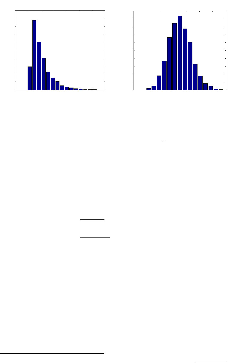
We illustrate the MMD density under both the null and alternative hypotheses by approximating it

empirically for p = q and p 6= q. Results are plotted in Figure 2.

Our goal is to determine whether the empirical test statistic MMD

is so large as to be outside

the 1−α quantile of the null distribution in (10), which gives a level α test. Consistency of this test

against local departures from the null hypothesis is provided by the following theorem, proved in

Appendix B.2.

Theorem 13 Deﬁne ρ

, ρ

, and t as in Theorem 12, and write µ

= µ

, where g

∈H is chosen

such that µ

remains a valid mean embedding, and

is made to approach zero as t →∞ to

describe local departures from the null hypothesis. Then

= ct

−1/2

is the minimum distance

between µ

and µ

distinguishable by the test.

An example of a local departure from the null hypothesis is described earlier in the discussion of

the L

distance between Parzen window estimates (Section 3.3.1). The class of local alternatives

considered in Theorem 13 is more general, however: for instance, Sriperumbudur et al. (2010b,

Section 4) and Harchaoui et al. (2008, Section 5, long version) give examples of classes of pertur-

bations g

with decreasing RKHS norm. These perturbations have the property that p differs from q

at increasing frequencies, rather than simply with decreasing amplitude.

One way to estimate the 1 −α quantile of the null distribution is using the bootstrap on the

aggregated data, following Arcones and Gin

e (1992). Alternatively, we may approximate the null

737

GRETTON, BORGWARDT, RASCH, SCH

OLKOPF AND SMOLA

−0.04 −0.02 0 0.02 0.04 0.06 0.08 0.1

Empirical MMD

density under H0

MMD

Prob. density

0.05 0.1 0.15 0.2 0.25 0.3 0.35 0.4

Empirical MMD

density under H1

MMD

Prob. density

Figure 2: Left: Empirical distribution of the MMD under H

, with p and q both Gaussians with

unit standard deviation, using 50 samples from each. Right: Empirical distribution of

the MMD under H

, with p a Laplace distribution with unit standard deviation, and q

a Laplace distribution with standard deviation 3

√

2, using 100 samples from each. In

both cases, the histograms were obtained by computing 2000 independent instances of

the MMD.

distribution by ﬁtting Pearson curves to its ﬁrst four moments (Johnson et al., 1994, Section 18.8).

Taking advantage of the degeneracy of the U-statistic, we obtain for m = n





MMD





m(m−1)

z,z

′



(z,z

′

)



and





MMD





8(m−2)

(m−1)

z,z

′



h(z,z

′

′′



h(z,z

′′

)h(z

′

′′

)



+ O(m

−4

) (11)

(see Appendix B.3), where h(z,z

′

) is deﬁned in Lemma 6, z = (x,y) ∼ p×q where x and y are inde-

pendent, and z

′

′′

are independent copies of z. The fourth moment E





MMD





is not computed,

since it is both very small, O(m

−4

), and expensive to calculate, O(m

). Instead, we replace the kur-

tosis

with a lower bound due to Wilkins (1944), kurt



MMD



≥



skew



MMD



+1. In Figure

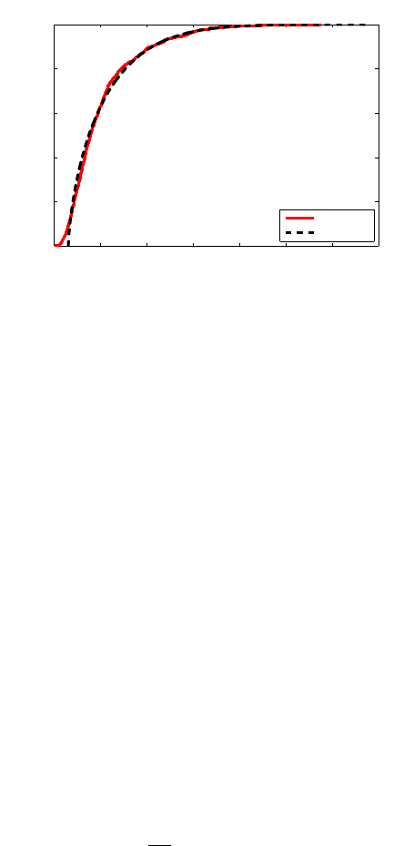
3, we illustrate the Pearson curve ﬁt to the null distribution: the ﬁt is good in the upper quantiles of

the distribution, where the test threshold is computed. Finally, we note that two alternative empiri-

cal estimates of the null distribution have more recently been proposed by Gretton et al. (2009): a

consistent estimate, based on an empirical computation of the eigenvalues λ

in (10); and an alter-

native Gamma approximation to the null distribution, which has a smaller computational cost but is

generally less accurate. Further detail and experimental comparisons are given by Gretton et al.

12. The kurtosis is deﬁned in terms of the fourth and second moments as kurt



MMD





[

MMD

]





[

MMD

]

i

−3.

738

A KERNEL TWO-SAMPLE TEST

−0.02 0 0.02 0.04 0.06 0.08 0.1 0.12

0.2

0.4

0.6

0.8

CDF of the MMD and Pearson fit

P(MMD

< t)

Emp. CDF

Pearson

Figure 3: Illustration of the empirical CDF of the MMD and a Pearson curve ﬁt. Both p and q were

Gaussian with zero mean and unit variance, and 50 samples were drawn from each. The

empirical CDF was computed on the basis of 1000 randomly generated MMD values. To

ensure the quality of ﬁt was determined only by the accuracy of the Pearson approxima-

tion, the moments used for the Pearson curves were also computed on the basis of these

1000 samples. The MMD used a Gaussian kernel with σ = 0.5.

6. A Linear Time Statistic and Test

The MMD-based tests are already more efﬁcient than the O(m

logm) and O(m

) tests described in

Section 3.3.3 (assuming m = n for conciseness). It is still desirable, however, to obtain O(m) tests

which do not sacriﬁce too much statistical power. Moreover, we would like to obtain tests which

have O(1) storage requirements for computing the test statistic, in order to apply the test to data

streams. We now describe how to achieve this by computing the test statistic using a subsampling

of the terms in the sum. The empirical estimate in this case is obtained by drawing pairs from X and

Y respectively without replacement.

Lemma 14 Deﬁne m

:= ⌊m/2⌋, assume m = n, and deﬁne h(z

) as in Lemma 6. The estimator

MMD

[F,X,Y] :=

∑

i=1

h((x

2i−1

),(x

))

can be computed in linear time, and is an unbiased estimate of MMD

[F, p, q].

While it is expected that MMD

has higher variance than MMD

(as we will see explicitly later), it

is computationally much more appealing. In particular, the statistic can be used in stream computa-

tions with need for only O(1) memory, whereas MMD

requires O(m) storage and O(m

) time to

compute the kernel h on all interacting pairs.

Since MMD

is just the average over a set of random variables, Hoeffding’s bound and the cen-

tral limit theorem readily allow us to provide both uniform convergence and asymptotic statements

with little effort. The ﬁrst follows directly from Hoeffding (1963, Theorem 2).

739

GRETTON, BORGWARDT, RASCH, SCH

OLKOPF AND SMOLA

Theorem 15 Assume 0 ≤ k(x

) ≤ K. Then

X,Y



MMD

(F,X,Y) −MMD

(F, p, q) > t



≤ exp



−t



where m

:= ⌊m/2⌋ (the same bound applies for deviations of −t and below).

Note that the bound of Theorem 10 is identical to that of Theorem 15, which shows the former is

rather loose. Next we invoke the central limit theorem (e.g., Serﬂing, 1980, Section 1.9).

Corollary 16 Assume 0 < E





< ∞. Then MMD

converges in distribution to a Gaussian ac-

cording to



MMD

−MMD

[F, p, q]



→ N



0,σ



where σ

= 2

z,z

′

(z,z

′

) −[E

z,z

′

h(z,z

′

)]

, where we use the shorthand E

z,z

′

:= E

z,z

′

∼p×q

The factor of 2 arises since we are averaging over only ⌊m/2⌋ observations. It is instructive to

compare this asymptotic distribution with that of the quadratic time statistic MMD

under H

when m = n. In this case, MMD

converges in distribution to a Gaussian according to



MMD

−MMD

[F, p, q]



→ N



0,σ



where σ

= 4





′

h(z,z

′

))



−[E

z,z

′

(h(z,z

′

))]



(Serﬂing, 1980, Section 5.5). Thus for MMD

the asymptotic variance is (up to scaling) the variance of E

′

[h(z,z

′

)], whereas for MMD

it is

Var

z,z

′

[h(z,z

′

)].

We end by noting another potential approach to reducing the cost of computing an empirical

MMD estimate, by using a low rank approximation to the Gram matrix (Fine and Scheinberg, 2001;

Williams and Seeger, 2001; Smola and Sch

olkopf, 2000). An incremental computation of the MMD

based on such a low rank approximation would require O(md) storage and O(md) computation

(where d is the rank of the approximate Gram matrix which is used to factorize both matrices)

rather than O(m) storage and O(m

) operations. That said, it remains to be determined what effect

this approximation would have on the distribution of the test statistic under H

, and hence on the

test threshold.

7. Related Metrics and Learning Problems

The present section discusses a number of topics related to the maximum mean discrepancy, includ-

ing metrics on probability distributions using non-RKHS function classes (Sections 7.1 and 7.2), the

relation with set kernels and kernels on probability measures (Section 7.3), an extension to kernel

measures of independence (Section 7.4), a two-sample statistic using a distribution over witness

functions (Section 7.5), and a connection to outlier detection (Section 7.6).

7.1 The MMD in Other Function Classes

The deﬁnition of the maximum mean discrepancy is by no means limited to RKHS. In fact, any

function class F that comes with uniform convergence guarantees and is sufﬁciently rich will enjoy

the above properties. Below, we consider the case where the scaled functions in F are dense inC(X)

(which is useful for instance when the functions in F are norm constrained).

740

A KERNEL TWO-SAMPLE TEST

Deﬁnition 17 Let F be a subset of some vector space. The star S[F] of a set F is

S[F] :=

{

αf|f ∈ F and α ∈[0,∞)

}

Theorem 18 Denote by F the subset of some vector space of functions from X to R for which

S[F] ∩C(X) is dense in C(X) with respect to the L

∞

(X) norm. Then MMD[F, p, q] = 0 if and only

if p = q, and MMD[F, p, q] is a metric on the space of probability distributions. Whenever the star

of F is not dense, the MMD deﬁnes a pseudo-metric space.

Proof It is clear that p = q implies MMD[F, p,q] = 0. The proof of the converse is very similar

to that of Theorem 5. Deﬁne H := S(F) ∩C(X). Since by assumption H is dense in C(X), there

exists an h

∗

∈ H satisfying

∗

− f

∞

< ε for all f ∈C(X). Write h

∗

:= α

∗

, where g

∗

∈ F. By

assumption, E

∗

−E

∗

= 0. Thus we have the bound

f(x) −E

( f(y))

≤

f(x) −E

∗

(x)

+ α

∗

(x) −E

∗

(y)

∗

(y) −E

f(y)

≤ 2ε

for all f ∈C(X) and ε > 0, which implies p = q by Lemma 1.

To show MMD[F, p, q] is a metric, it remains to prove the triangle inequality. We have

sup

f∈F



f −E



+ sup

g∈F



g−E



≥ sup

f∈F





f −E



f −E





≥ sup

f∈F

f −E

Note that any uniform convergence statements in terms of F allow us immediately to characterize

an estimator of MMD(F, p,q) explicitly. The following result shows how (this reasoning is also the

basis for the proofs in Section 4, although here we do not restrict ourselves to an RKHS).

Theorem 19 Let δ ∈(0, 1) be a conﬁdence level and assume that for some ε(δ,m, F) the following

holds for samples

{

,.. .,x

}

drawn from p:

(

sup

f∈F



[ f] −

∑

i=1

f(x

)



> ε(δ,m,F)

)

≤ δ.

In this case we have that,

X,Y

MMD[F, p, q] −MMD

[F,X,Y]

> 2ε(δ/2,m,F)

}

≤ δ,

where MMD

[F,X,Y] is taken from Deﬁnition 2.

Proof The proof works simply by using convexity and suprema as follows:

MMD[F, p, q] −MMD

[F,X,Y]



sup

f∈F

[ f] −E

[ f]

−sup

f∈F



∑

i=1

f(x

) −

∑

i=1

f(y

)



≤sup

f∈F



[ f] −E

[ f] −

∑

i=1

f(x

) +

∑

i=1

f(y

)



≤sup

f∈F



[ f] −

∑

i=1

f(x

)



+ sup

f∈F



[ f] −

∑

i=1

f(y

)



741

GRETTON, BORGWARDT, RASCH, SCH

OLKOPF AND SMOLA

Bounding each of the two terms via a uniform convergence bound proves the claim.

This shows that MMD

[F,X,Y] can be used to estimate MMD[F, p, q], and that the quantity is

asymptotically unbiased.

Remark 20 (Reduction to Binary Classiﬁcation) As noted by Friedman (2003), any classiﬁer

which maps a set of observations

{

}

with z

∈ X on some domain X and labels l

∈

{

±1

}

, for

which uniform convergence bounds exist on the convergence of the empirical loss to the expected

loss, can be used to obtain a similarity measure on distributions—simply assign l

= 1 if z

∈ X and

= −1 for z

∈Y and ﬁnd a classiﬁer which is able to separate the two sets. In this case maxi-

mization of E

[ f] −E

[ f] is achieved by ensuring that as many z ∼ p(z) as possible correspond to

f(z) = 1, whereas for as many z ∼ q(z) as possible we have f(z) = −1. Consequently neural net-

works, decision trees, boosted classiﬁers and other objects for which uniform convergence bounds

can be obtained can be used for the purpose of distribution comparison. Metrics and divergences

on distributions can also be deﬁned explicitly starting from classiﬁers. For instance, Sriperumbudur

et al. (2009, Section 2) show the MMD minimizes the expected risk of a classiﬁer with linear loss

on the samples X and Y, and Ben-David et al. (2007, Section 4) use the error of a hyperplane clas-

siﬁer to approximate the A-distance between distributions (Kifer et al., 2004). Reid and Williamson

(2011) provide further discussion and examples.

7.2 Examples of Non-RKHS Function Classes

Other function spaces F inspired by the statistics literature can also be considered in deﬁning the

MMD. Indeed, Lemma 1 deﬁnes an MMD with F the space of bounded continuous real-valued

functions, which is a Banach space with the supremum norm (Dudley, 2002, p. 158). We now

describe two further metrics on the space of probability distributions, namely the Kolmogorov-

Smirnov and Earth Mover’s distances, and their associated function classes.

7.2.1 KOLMOGOROV-SMIRNOV STATISTIC

The Kolmogorov-Smirnov (K-S) test is probably one of the most famous two-sample tests in statis-

tics. It works for random variables x ∈ R (or any other set for which we can establish a total order).

Denote by F

(x) the cumulative distribution function of p and let F

(x) be its empirical counterpart,

(z) := Pr

{

x ≤ z for x ∼ p

}

and F

(z) :=

|X|

∑

i=1

z≤x

It is clear that F

captures the properties of p. The Kolmogorov metric is simply the L

∞

distance

−F

∞

for two sets of observations X and Y. Smirnov (1939) showed that for p = q the limiting

distribution of the empirical cumulative distribution functions satisﬁes

lim

m,n→∞

X,Y



m+n



−F

∞

> x

= 2

∞

∑

j=1

(−1)

j−1

−2j

for x ≥ 0, (12)

which is distribution independent. This allows for an efﬁcient characterization of the distribution

under the null hypothesis H

. Efﬁcient numerical approximations to (12) can be found in numerical

analysis handbooks (Press et al., 1994). The distribution under the alternative p 6= q, however, is

unknown.

742

A KERNEL TWO-SAMPLE TEST

The Kolmogorov metric is, in fact, a special instance of MMD[F, p, q] for a certain Banach

space (M

uller, 1997, Theorem 5.2).

Proposition 21 Let F be the class of functions X → R of bounded variation

1. Then

MMD[F, p, q] =



−F



∞

7.2.2 EARTH-MOVER DISTANCES

Another class of distance measures on distributions that may be written as maximum mean discrep-

ancies are the Earth-Mover distances. We assume (X, ρ) is a separable metric space, and deﬁne

(X) to be the space of probability measures on X for which

ρ(x,z)dp(z) < ∞ for all p ∈P

(X)

and x ∈ X (these are the probability measures for which E

< ∞ when X = R). We then have the

following deﬁnition (Dudley, 2002, p. 420).

Deﬁnition 22 (Monge-Wasserstein metric) Let p ∈P

(X) and q ∈P

(X). The Monge-Wasserstein

distance is deﬁned as

W(p,q) := inf

µ∈M(p,q)

ρ(x,y)dµ(x,y),

where M(p, q) is the set of joint distributions on X ×X with marginals p and q.

We may interpret this as the cost (as represented by the metric ρ(x, y)) of transferring mass dis-

tributed according to p to a distribution in accordance with q, where µ is the movement schedule.

In general, a large variety of costs of moving mass from x to y can be used, such as psycho-optical

similarity measures in image retrieval (Rubner et al., 2000). The following theorem provides the

link with the MMD (Dudley, 2002, Theorem 11.8.2).

Theorem 23 (Kantorovich-Rubinstein) Let p ∈ P

(X) and q ∈ P

(X), where X is separable.

Then a metric on P

(S) is deﬁned as

W(p,q) =

p−q

∗

= sup

≤1



f d(p−q)



where

:= sup

x6=y∈X

f(x) − f(y)

ρ(x,y)

is the Lipschitz seminorm

for real valued f on X.

A simple example of this theorem is as follows (Dudley, 2002, Exercise 1, p. 425).

Example 2 Let X = R with associated ρ(x, y) =

x−y

. Then given f such that

≤ 1, we use

integration by parts to obtain



f d(p−q)



−F

)(x) f

′

(x)dx



≤



−F

)



(x)dx,

13. A function f deﬁned on [a, b] is of bounded variation C if the total variation is bounded by C, that is, the supremum

over all sums

∑

1≤i≤n

|f (x

) − f(x

i−1

)|,

where a ≤x

≤ ... ≤ x

≤ b (Dudley, 2002, p. 184).

14. A seminorm satisﬁes the requirements of a norm besides

= 0 only for x = 0 (Dudley, 2002, p. 156).

743

GRETTON, BORGWARDT, RASCH, SCH

OLKOPF AND SMOLA

where the maximum is attained for the function g with derivative g

′

= 21

−1 (and for which

= 1). We recover the L

distance between distribution functions,

W(P,Q) =



−F

)



(x)dx.

One may further generalize Theorem 23 to the set of all laws P(X) on arbitrary metric spaces X

(Dudley, 2002, Proposition 11.3.2).

Deﬁnition 24 (Bounded Lipschitz metric) Let p and q be laws on a metric space X. Then

β(p,q) := sup

≤1



f d(p−q)



is a metric on P(X), where f belongs to the space of bounded Lipschitz functions with norm

∞

Empirical estimates of the Monge-Wasserstein and Bounded Lipschitz metrics on R

are provided

by Sriperumbudur et al. (2010a).

7.3 Set Kernels and Kernels Between Probability Measures

artner et al. (2002) propose kernels for Multi-Instance Classiﬁcation (MIC) which deal with sets of

observations. The purpose of MIC is to ﬁnd estimators which are able to infer that if some elements

in a set satisfy a certain property, then the set of observations also has this property. For instance,

a dish of mushrooms is poisonous if it contains any poisonous mushrooms. Likewise a keyring

will open a door if it contains a suitable key. One is only given the ensemble, however, rather than

information about which instance of the set satisﬁes the property.

The solution proposed by G

artner et al. (2002) is to map the ensembles X

{

,.. .,x

}

where i is the ensemble index and m

the number of elements in the ith ensemble, jointly into

feature space via

φ(X

) :=

∑

j=1

φ(x

and to use the latter as the basis for a kernel method. This simple approach affords rather good

performance. With the beneﬁt of hindsight, it is now understandable why the kernel

k(X

) =

∑

u,v

k(x

)

produces useful results: it is simply the kernel between the empirical means in feature space



µ(X

),µ(X

)



(Hein et al., 2004, Equation 4). Jebara and Kondor (2003) later extended this set-

ting by smoothing the empirical densities before computing inner products.

Note, however, that the empirical mean embedding µ

may not be the best statistic to use for

MIC: we are only interested in determining whether some instances in the domain have the desired

property, rather than making a statement regarding the distribution over all instances. Taking this

into account leads to an improved algorithm (Andrews et al., 2003).

744

A KERNEL TWO-SAMPLE TEST

7.4 Kernel Measures of Independence

We next demonstrate the application of MMD in determining whether two random variables x and

y are independent. In other words, assume that pairs of random variables (x

) are jointly drawn

from some distribution p := p

. We wish to determine whether this distribution factorizes; that

is, whether q := p

× p

is the same as p. One application of such an independence measure is in

independent component analysis (Comon, 1994), where the goal is to ﬁnd a linear mapping of the

observations x

to obtain mutually independent outputs. Kernel methods were employed to solve

this problem by Bach and Jordan (2002), Gretton et al. (2005a,b), and Shen et al. (2009). In the

following we re-derive one of the above kernel independence measures as a distance between mean

embeddings (see also Smola et al., 2007).

We begin by deﬁning

µ[p

] := E

x,y

[v((x,y), ·)]

and µ[p

× p

] := E

[v((x,y), ·)].

Here we assume V is an RKHS over X×Y with kernel v((x,y), (x

′

)). If x and y are dependent, then

µ[p

] 6= µ[p

×p

]. Hence we may use ∆(V, p

, p

×p

) :=

µ[p

] −µ[p

× p

]

as a measure of

dependence.

Now assume that v((x,y),(x

′

)) = k(x,x

′

)l(y,y

′

), that is, the RKHS V is a direct product H ⊗G

of RKHSs on X and Y. In this case it is easy to see that

∆

(V, p

, p

× p

) =

[k(x, ·)l(y, ·)]−E

[k(x, ·)]E

[l(y,·)]

= E

′



k(x, x

′

)l(y,y

′

)



−2E

′



k(x, x

′

)l(y,y

′

)



′



k(x, x

′

)l(y,y

′

)



The latter is also the squared Hilbert-Schmidt norm of the cross-covariance operator between RKHSs

(Gretton et al., 2005a): for characteristic kernels, this is zero if and only if x and y are independent.

Theorem 25 Denote by C

the covariance operator between random variables x and y, drawn

jointly from p

, where the functions on X and Y are the reproducing kernel Hilbert spaces F and G

respectively. Then the Hilbert-Schmidt norm

equals ∆(V, p

, p

× p

Empirical estimates of this quantity are as follows:

Theorem 26 Denote by K and L the kernel matrices on X and Y respectively, and by H = I −1/m

the projection matrix onto the subspace orthogonal to the vector with all entries set to 1 (where 1 is

an m×m matrix of ones). Then m

−2

trHKHL is an estimate of ∆

with bias O(m

−1

). The deviation

from ∆

is O

−1/2

Gretton et al. (2005a) provide explicit constants. In certain circumstances, including in the case of

RKHSs with Gaussian kernels, the empirical ∆

may also be interpreted in terms of a smoothed

difference between the joint empirical characteristic function (ECF) and the product of the marginal

ECFs (Feuerverger, 1993; Kankainen, 1995). This interpretation does not hold in all cases, however,

for example, for kernels on strings, graphs, and other structured spaces. An illustration of the wit-

ness function f

∗

∈V from Section 2.3 is provided in Figure 4, for the case of dependence detection.

This is a smooth function which has large magnitude where the joint density is most different from

the product of the marginals.

745

GRETTON, BORGWARDT, RASCH, SCH

OLKOPF AND SMOLA

Dependence witness and sample

−1.5 −1 −0.5 0 0.5 1 1.5

−1.5

−1

−0.5

0.5

1.5

−0.04

−0.03

−0.02

−0.01

0.01

0.02

0.03

0.04

0.05

Figure 4: Illustration of the function maximizing the mean discrepancy when MMD is used as a

measure of dependence. A sample from dependent random variables x and y is shown

in black, and the associated function

∗

that witnesses the MMD is plotted as a contour.

The latter was computed empirically on the basis of 200 samples, using a Gaussian kernel

with σ = 0.2.

We remark that a hypothesis test based on the above kernel statistic is more complicated than

for the two-sample problem, since the product of the marginal distributions is in effect simulated

by permuting the variables of the original sample. Further details are provided by Gretton et al.

(2008b).

7.5 Kernel Statistics Using a Distribution over Witness Functions

Shawe-Taylor and Dolia (2007) deﬁne a distance between distributions as follows: let H be a set of

functions on X and r be a probability distribution over H. Then the distance between two distribu-

tions p and q is given by

D(p,q) := E

f∼r( f)

[ f(x)] −E

[ f(y)]

. (13)

746

A KERNEL TWO-SAMPLE TEST

That is, we compute the average distance between p and q with respect to a distribution over test

functions. The following result shows the relation with the MMD, and is due to Song et al. (2008,

Section 6).

Lemma 27 Let H be a reproducing kernel Hilbert space, f ∈H, and assume r( f) = r(

) with

ﬁnite E

f∼r

[kfk

]. Then D(p,q) = C



−µ



for some constant C which depends only on H

and r.

Proof By deﬁnition E

[ f(x)] =

, f

. Using linearity of the inner product, Equation (13) equals





−µ

, f





dr( f)



−µ





−µ



−µ



, f



dr( f),

where the integral is independent of p,q. To see this, note that for any p, q,

−µ

is a unit vector

which can be transformed into the ﬁrst canonical basis vector (for instance) by a rotation which

leaves the integral invariant, bearing in mind that r is rotation invariant.

7.6 Outlier Detection

An application related to the two sample problem is that of outlier detection: this is the question of

whether a novel point is generated from the same distribution as a particular i.i.d. sample. In a way,

this is a special case of a two sample test, where the second sample contains only one observation.

Several methods essentially rely on the distance between a novel point to the sample mean in feature

space to detect outliers.

For instance, Davy et al. (2002) use a related method to deal with nonstationary time series.

Likewise Shawe-Taylor and Cristianini (2004, p. 117) discuss how to detect novel observations by

using the following reasoning: the probability of being an outlier is bounded both as a function of

the spread of the points in feature space and the uncertainty in the empirical feature space mean (as

bounded using symmetrisation and McDiarmid’s tail bound).

Instead of using the sample mean and variance, Tax and Duin (1999) estimate the center and

radius of a minimal enclosing sphere for the data, the advantage being that such bounds can po-

tentially lead to more reliable tests for single observations. Sch

olkopf et al. (2001) show that the

minimal enclosing sphere problem is equivalent to novelty detection by means of ﬁnding a hyper-

plane separating the data from the origin, at least in the case of radial basis function kernels.

8. Experiments

We conducted distribution comparisons using our MMD-based tests on data sets from three real-

world domains: database applications, bioinformatics, and neurobiology. We investigated both

uniform convergence approaches (MMD

with the Corollary 9 threshold, and MMD

H with the

Corollary 11 threshold); the asymptotic approaches with bootstrap (MMD

B) and moment match-

ing to Pearson curves (MMD

M), both described in Section 5; and the asymptotic approach using

the linear time statistic (MMD

) from Section 6. We also compared against several alternatives from

747

GRETTON, BORGWARDT, RASCH, SCH

OLKOPF AND SMOLA

the literature (where applicable): the multivariate t-test, the Friedman-Rafsky Kolmogorov-Smirnov

generalisation (Smir), the Friedman-Rafsky Wald-Wolfowitz generalisation (Wolf), the Biau-Gy

orﬁ

test (Biau) with a uniform space partitioning, and the Hall-Tajvidi test (Hall). See Section 3.3 for

details regarding these tests. Note that we do not apply the Biau-Gy

orﬁ test to high-dimensional

problems (since the required space partitioning is no longer possible), and that MMD is the only

method applicable to structured data such as graphs.

An important issue in the practical application of the MMD-based tests is the selection of the

kernel parameters. We illustrate this with a Gaussian RBF kernel, where we must choose the kernel

width σ (we use this kernel for univariate and multivariate data, but not for graphs). The empirical

MMD is zero both for kernel size σ = 0 (where the aggregate Gram matrix over X and Y is a unit

matrix), and also approaches zero as σ →∞ (where the aggregate Gram matrix becomes uniformly

constant). We set σ to be the median distance between points in the aggregate sample, as a compro-

mise between these two extremes: this remains a heuristic, similar to those described in Takeuchi

et al. (2006) and Sch

olkopf (1997), and the optimum choice of kernel size is an ongoing area of

research. We further note that setting the kernel using the sample being tested may cause changes to

the asymptotic distribution: in particular, the analysis in Sections 4 and 5 assumes the kernel not to

be a function of the sample. An analysis of the convergence of MMD when the kernel is adapted on

the basis of the sample is provided by Sriperumbudur et al. (2009), although the asymptotic distri-

bution in this case remains a topic of research. As a practical matter, however, the median heuristic

has not been observed to have much effect on the asymptotic distribution, and in experiments is

indistinguishable from results obtained by computing the kernel on a small subset of the sample set

aside for this purpose. See Appendix C for more detail.

8.1 Toy Example: Two Gaussians

In our ﬁrst experiment, we investigated the scaling performance of the various tests as a function

of the dimensionality d of the space X ⊂ R

, when both p and q were Gaussian. We considered

values of d up to 2500: the performance of the MMD-based tests cannot therefore be explained

in the context of density estimation (as in Section 3.3.1), since the associated density estimates are

necessarily meaningless here. The levelsfor all tests were set at α = 0.05, m = n = 250 samples were

used, and results were averaged over 100 repetitions. In the ﬁrst case, the distributions had different

means and unit variance. The percentage of times the null hypothesis was correctly rejected over a

set of Euclidean distances between the distribution means (20 values logarithmically spaced from

0.05 to 50), was computed as a function of the dimensionality of the normal distributions. In case

of the t-test, a ridge was added to the covariance estimate, to avoid singularity (the ratio of largest

to smallest eigenvalue was ensured to be at most 2). In the second case, samples were drawn from

distributions N(0,I) and N(0,σ

I) with different variance. The percentage of null rejections was

averaged over 20 σ values logarithmically spaced from 10

0.01

to 10. The t-test was not compared in

this case, since its output would have been irrelevant. Results are plotted in Figure 5.

In the case of Gaussians with differing means, we observe the t-test performs best in low di-

mensions, however its performance is severely weakened when the number of samples exceeds the

number of dimensions. The performance of MMD

M is comparable to the t-test in low dimen-

sions, and outperforms all other methods in high dimensions. The worst performance is obtained

for MMD

H, though MMD

also does relatively poorly: this is unsurprising given that these tests

748

A KERNEL TWO-SAMPLE TEST

A B

0.2

0.4

0.6

0.8

Dimension

Normal dist. having different variances

0.2

0.4

0.6

0.8

Dimension

percent correctly rejecting H

Normal dist. having different means

MMD

t−test

FR Wolf

FR Smirnov

Hall

Figure 5: Type II performance of the various tests when separating two Gaussians, with test level

α = 0.05. A Gaussians having same variance and different means. B Gaussians having

same mean and different variances.

derive from distribution-free large deviation bounds, and the sample size is relatively small. Re-

markably, MMD

performs quite well compared with the Section 3.3.3 tests in high dimensions.

In the case of Gaussians of differing variance, the Hall test performs best, followed closely

by MMD

M. FR Wolf and (to a much greater extent) FR Smirnov both have difﬁculties in high

dimensions, failing completely once the dimensionality becomes too great. The linear-cost test

MMD

again performs surprisingly well, almost matching the MMD

M performance at the highest

dimensionality. Both MMD

H and MMD

perform poorly, the former failing completely: this

is one of several illustrations we will encounter of the much greater tightness of the Corollary 9

threshold over that in Corollary 11.

8.2 Data Integration

In our next application of MMD, we performed distribution testing for data integration: the objec-

tive being to aggregate two data sets into a single sample, with the understanding that both original

samples were generated from the same distribution. Clearly, it is important to check this last con-

dition before proceeding, or an analysis could detect patterns in the new data set that are caused

by combining the two different source distributions. We chose several real-world settings for this

task: we compared microarray data from normal and tumor tissues (Health status), microarray data

from different subtypes of cancer (Subtype), and local ﬁeld potential (LFP) electrode recordings

from the Macaque primary visual cortex (V1) with and without spike events (Neural Data I and

II, as described in more detail by Rasch et al., 2008). In all cases, the two data sets have different

statistical properties, but the detection of these differences is made difﬁcult by the high data dimen-

sionality (indeed, for the microarray data, density estimation is impossible given the sample size and

data dimensionality, and no successful test can rely on accurate density estimates as an intermediate

step).

749

GRETTON, BORGWARDT, RASCH, SCH

OLKOPF AND SMOLA

Data Set Attr. MMD

MMD

H MMD

B MMD

M t-test Wolf Smir Hall

Neural Data I Same 100.0 100.0 96.5 96.5 100.0 97.0 95.0 96.0

Different 38.0 100.0 0.0 0.0 42.0 0.0 10.0 49.0

Neural Data II Same 100.0 100.0 94.6 95.2 100.0 95.0 94.5 96.0

Different 99.7 100.0 3.3 3.4 100.0 0.8 31.8 5.9

Health status Same 100.0 100.0 95.5 94.4 100.0 94.7 96.1 95.6

Different 100.0 100.0 1.0 0.8 100.0 2.8 44.0 35.7

Subtype Same 100.0 100.0 99.1 96.4 100.0 94.6 97.3 96.5

Different 100.0 100.0 0.0 0.0 100.0 0.0 28.4 0.2

Table 1: Distribution testing for data integration on multivariate data. Numbers indicate the per-

centage of repetitions for which the null hypothesis (p=q) was accepted, given α = 0.05.

Sample size (dimension; repetitions of experiment): Neural I 4000 (63; 100) ; Neural II

1000 (100; 1200); Health Status 25 (12,600; 1000); Subtype 25 (2,118; 1000).

Data Set Attr. MMD

MMD

H MMD

B MMD

M t-test Wolf Smir Hall Biau

BIO Same 100.0 100.0 93.8 94.8 95.2 90.3 95.8 95.3 99.3

Different 20.0 52.6 17.2 17.6 36.2 17.2 18.6 17.9 42.1

FOREST Same 100.0 100.0 96.4 96.0 97.4 94.6 99.8 95.5 100.0

Different 3.9 11.0 0.0 0.0 0.2 3.8 0.0 50.1 0.0

CNUM Same 100.0 100.0 94.5 93.8 94.0 98.4 97.5 91.2 98.5

Different 14.9 52.7 2.7 2.5 19.17 22.5 11.6 79.1 50.5

FOREST10D Same 100.0 100.0 94.0 94.0 100.0 93.5 96.5 97.0 100.0

Different 86.6 100.0 0.0 0.0 0.0 0.0 1.0 72.0 100.0

Table 2: Naive attribute matching on univariate (BIO, FOREST, CNUM) and multivariate (FOR-

EST10D) data. Numbers indicate the percentage of times the null hypothesis p = q was

accepted with α = 0.05, pooled over attributes. Sample size (dimension; attributes; repeti-

tions of experiment): BIO 377 (1; 6; 100); FOREST 538 (1; 10; 100); CNUM 386 (1; 13;

100); FOREST10D 1000 (10; 2; 100).

We applied our tests to these data sets in the following fashion. Given two data sets A and B,

we either chose one sample from A and the other from B (attributes = different); or both samples

from either A or B (attributes = same). We then repeated this process up to 1200 times. Results

are reported in Table 1. Our asymptotic tests perform better than all competitors besides Wolf : in

the latter case, we have greater Type II error for one neural data set, lower Type II error on the

Health Status data (which has very high dimension and low sample size), and identical (error-free)

performance on the remaining examples. We note that the Type I error of the bootstrap test on the

Subtype data set is far from its design value of 0.05, indicating that the Pearson curves provide a

better threshold estimate for these low sample sizes. For the remaining data sets, the Type I errors

of the Pearson and Bootstrap approximations are close. Thus, for larger data sets, the bootstrap is

to be preferred, since it costs O(m

), compared with a cost of O(m

) for the Pearson curves (due to

the cost of computing (11)). Finally, the uniform convergence-based tests are too conservative, with

MMD

ﬁnding differences in distribution only for the data with largest sample size, and MMD

never ﬁnding differences.

750

A KERNEL TWO-SAMPLE TEST

8.3 Computational Cost

We next investigate the tradeoff between computational cost and performance of the various tests,

with a particular focus on how the quadratic-cost MMD tests from Sections 4 and 5 compare with the

linear time MMD-based asymptotic test from Section 6. We consider two 1-D data sets (CNUM and

FOREST) and two higher-dimensional data sets (FOREST10D and NEUROII). Results are plotted

in Figure 6. If cost is not a factor, then the MMD

B shows best overall performance as a function

of sample size, with a Type II error dropping to zero as fast or faster than competing approaches in

three of four cases, and narrowly trailing FR Wolf in the remaining case (FOREST10D). That said,

for data sets CNUM, FOREST, and FOREST10D, the linear time MMD achieves a given Type II

error at a far smaller computational cost than MMD

B, albeit by looking at a great deal more data.

In the CNUM case, however, the linear test is not able to achieve zero error even for the largest

data set size. For the NEUROII data, attaining zero Type II error has about the same cost for both

approaches. The difference in cost of MMD

B and MMD

is due to the bootstrapping required for

the former, which produces a constant offset in cost between the two (here 150 resamplings were

used).

The t-test also performs well in three of the four problems, and in fact represents the best cost-

performance tradeoff in these three data sets (i.e., while it requires much more data than MMD

for a given Type II error rate, it costs far less to compute). The t-test assumes that only the difference

in means is important in distinguishing the distributions, and it requires an accurate estimate of

the within-sample covariance; the test fails completely on the NEUROII data. We emphasise that

the Kolmogorov-Smirnov results in 1-D were obtained using the classical statistic, and not the

Friedman-Rafsky statistic, hence the low computational cost. The cost of both Friedman-Rafsky

statistics is therefore given by the FR Wolf cost in this case. The latter scales similarly with sample

size to the quadratic time MMD tests, conﬁrming Friedman and Rafsky’s observation that obtaining

the pairwise distances between sample points is the dominant cost of their tests. We also remark

on the unusual behaviour of the Type II error of the FR Wolf test in the FOREST data set, which

worsens for increasing sample size.

We conclude that the approach to be recommended for two-sample testing will depend on the

data available: for small amounts of data, the best results are obtained using every observation to

maximum effect, and employing the quadratic time MMD

B test. When large volumes of data are

available, a better option is to look at each point only once, which can yield lower Type II error for a

given computational cost. It may also be worth doing a t-test ﬁrst in this case, and only running more

sophisticated nonparametric tests if the t-test accepts the null hypothesis, to verify the distributions

are identical in more than just mean.

8.4 Attribute Matching

Our ﬁnal series of experiments addresses automatic attribute matching. Given two databases, we

want to detect corresponding attributes in the schemas of these databases, based on their data-

content (as a simple example, two databases might have respective ﬁelds Wage and Salary, which are

assumed to be observed via a subsampling of a particular population, and we wish to automatically

determine that both Wage and Salary denote to the same underlying attribute). We use a two-

sample test on pairs of attributes from two databases to ﬁnd corresponding pairs.

This procedure

15. Note that corresponding attributes may have different distributions in real-world databases. Hence, schema matching

cannot solely rely on distribution testing.

751

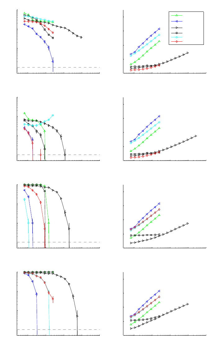
GRETTON, BORGWARDT, RASCH, SCH

OLKOPF AND SMOLA

−3

−2

−1

Type II error

Sample #

Dataset: CNUM

−4

−2

Time per test [sec]

Sample #

Dataset: CNUM

MMD

t−test

FR Wolf

FR Smir

−3

−2

−1

Type II error

Sample #

Dataset: FOREST

−4

−2

Time per test [sec]

Sample #

Dataset: FOREST

−3

−2

−1

Type II error

Sample #

Dataset: FOREST10D

−4

−2

Time per test [sec]

Sample #

Dataset: FOREST10D

−3

−2

−1

Type II error

Sample #

Dataset: NEUROII

−4

−2

Time per test [sec]

Sample #

Dataset: NEUROII

Figure 6: Linear-cost vs quadratic-cost MMD. The ﬁrst column shows Type II performance, and

the second shows runtime. The dashed grey horizontal line indicates zero Type II error

(required due to log y-axis).

752

A KERNEL TWO-SAMPLE TEST

is also called table matching for tables from different databases. We performed attribute matching

as follows: ﬁrst, the data set D was split into two halves A and B. Each of the n attributes in A (and

B, resp.) was then represented by its instances in A (resp. B). We then tested all pairs of attributes

from A and from B against each other, to ﬁnd the optimal assignment of attributes A

,.. .,A

from

A to attributes B

,.. .,B

from B. We assumed that A and B contain the same number of attributes.

As a naive approach, we could assume that any possible pair of attributes might correspond,

and thus that every attribute of A needs to be tested against all the attributes of B to ﬁnd the opti-

mal match. We report results for this naive approach, aggregated over all pairs of possible attribute

matches, in Table 2. We used three data sets: the census income data set from the UCI KDD archive

(CNUM), the protein homology data set from the 2004 KDD Cup (BIO) (Caruana and Joachims,

2004), and the forest data set from the UCI ML archive (Blake and Merz, 1998). For the ﬁnal data

set, we performed univariate matching of attributes (FOREST) and multivariate matching of tables

(FOREST10D) from two different databases, where each table represents one type of forest. Both

our asymptotic MMD

-based tests perform as well as or better than the alternatives, notably for

CNUM, where the advantage of MMD

is large. Unlike in Table 1, the next best alternatives are not

consistently the same across all data: for example, in BIO they are Wolf or Hall, whereas in FOR-

EST they are Smir, Biau, or the t-test. Thus, MMD

appears to perform more consistently across

the multiple data sets. The Friedman-Rafsky tests do not always return a Type I error close to the

design parameter: for instance, Wolf has a Type I error of 9.7% on the BIO data set (on these data,

MMD

has the joint best Type II error without compromising the designed Type I performance).

Finally, MMD

performs much better than in Table 1, although surprisingly it fails to reliably detect

differences in FOREST10D. The results of MMD

H are also improved, although it remains among

the worst performing methods.

A more principled approach to attribute matching is also possible. Assume that

φ(A) = (φ

),φ

),..., φ

)): in other words, the kernel decomposes into kernels on the indi-

vidual attributes of A (and also decomposes this way on the attributes of B). In this case, MMD

can

be written

∑

i=1

kµ

) −µ

, where we sum over the MMD terms on each of the attributes.

Our goal of optimally assigning attributes from B to attributes of A via MMD is equivalent to ﬁnding

the optimal permutation π of attributes of B that minimizes

∑

i=1

kµ

) −µ

π(i)

. If we deﬁne

= kµ

) −µ

, then this is the same as minimizing the sum over C

i,π(i)

. This is the linear

assignment problem, which costs O(n

) time using the Hungarian method (Kuhn, 1955).

While this may appear to be a crude heuristic, it nonetheless deﬁnes a semi-metric on the sample

spaces X andY and the corresponding distributions p and q. This follows from the fact that matching

distances are proper metrics if the matching cost functions are metrics. We formalize this as follows:

Theorem 28 Let p, q be distributions on R

and denote by p

the marginal distributions on the

i-th variable. Moreover, denote by Π the symmetric group on

{

1,.. .,d

}

. The following distance,

obtained by optimal coordinate matching, is a semi-metric.

∆[F, p, q] := min

π∈Π

∑

i=1

MMD[F, p

π(i)

Proof Clearly ∆[F, p, q] is nonnegative, since it is a sum of nonnegative quantities. Next we show

the triangle inequality. Denote by r a third distribution on R

and let π

p,q

,π

q,r

and π

p,r

be the

753

GRETTON, BORGWARDT, RASCH, SCH

OLKOPF AND SMOLA

distance minimizing permutations over the associated pairs from {p,q, r}. It follows that

∆[F, p, q] +∆[F,q,r] =

∑

i=1

MMD[F, p

p,q

(i)

] +

∑

i=1

MMD[F,q

q,r

(i)

]

≥

∑

i=1

MMD[F, p

[π

p,q

◦π

q,r

](i)

] ≥ ∆[F, p, r].

The ﬁrst inequality follows from the triangle inequality on MMD,

MMD[F, p

p,q

(i)

] + MMD[F, q

p,q

(i)

[π

p,q

◦π

q,r

](i)

] ≥ MMD[F, p

[π

p,q

◦π

q,r

](i)

The second inequality is a result of minimization over π.

We tested this ’Hungarian approach’ to attribute matching via MMD

B on three univariate

data sets (BIO, CNUM, FOREST) and for table matching on a fourth (FOREST10D). To study

MMD

B on structured data, we used two data sets of protein graphs (PROTEINS and ENZYMES)

and used the graph kernel for proteins from Borgwardt et al. (2005) for table matching via the

Hungarian method (the other tests were not applicable to these graph data). The challenge here is

to match tables representing one functional class of proteins (or enzymes) from data set A to the

corresponding tables (functional classes) in B. Results are shown in Table 3. Besides on the BIO

and CNUM data sets, MMD

B made no errors.

Data Set Data type No. attributes Sample size Repetitions % correct

BIO univariate 6 377 100 90.0

CNUM univariate 13 386 100 99.8

FOREST univariate 10 538 100 100.0

FOREST10D multivariate 2 1000 100 100.0

ENZYME structured 6 50 50 100.0

PROTEINS structured 2 200 50 100.0

Table 3: Hungarian Method for attribute matching via MMD

B on univariate (BIO, CNUM,

FOREST), multivariate (FOREST10D), and structured (ENZYMES, PROTEINS) data

(α = 0.05; “% correct” is the percentage of correct attribute matches over all repetitions).

9. Conclusion

We have established three simple multivariate tests for comparing two distributions p and q, based

on samples of size m and n from these respective distributions. Our test statistic is the maximum

mean discrepancy (MMD), deﬁned as the maximum deviation in the expectation of a function eval-

uated on each of the random variables, taken over a sufﬁciently rich function class: in our case, a

reproducing kernel Hilbert space (RKHS). Equivalently, the statistic can be written as the norm of

the difference between distribution feature means in the RKHS. We do not require density estimates

as an intermediate step. Two of our tests provide Type I error bounds that are exact and distribution-

free for ﬁnite sample sizes. We also give a third test based on quantiles of the asymptotic distribution

754

A KERNEL TWO-SAMPLE TEST

of the associated test statistic. All three tests can be computed in O((m+ n)

) time, however when

sufﬁcient data are available, a linear time statistic can be used, which in our experiments was able to

achieve a given Type II error at smaller computational cost, by looking at many more samples than

the quadratic-cost tests.

We have seen in Section 7 that several classical metrics on probability distributions can be writ-

ten as integral probability metrics with function classes that are not Hilbert spaces, but rather Banach

or seminormed spaces (for instance the Kolmogorov-Smirnov and Earth Mover’s distances). It is

therefore of interest to establish under what conditions one could write these discrepancies in terms

of norms of differences of mean embeddings. Sriperumbudur et al. (2011b) provide expressions

for the maximum mean discrepancy in terms of mean embeddings in reproducing kernel Banach

spaces. When the Banach space is not an RKBS, the question of establishing a mean embedding

interpretation for the MMD remains open.

We also note (following Section 7.3) that the MMD for RKHSs is associated with a particular

kernel between probability distributions. Hein et al. (2004) describe several further such kernels,

which induce corresponding distances between feature space distribution mappings: these may in

turn lead to new and powerful two-sample tests.

Two recent studies have shown that additional divergence measures between distributions can

be obtained empirically through optimization in a reproducing kernel Hilbert space. Harchaoui

et al. (2008) deﬁne a two-sample test statistic arising from the kernel Fisher discriminant, rather

than the difference of RKHS means; and Nguyen et al. (2008) obtain a KL divergence estimate

by approximating the ratio of densities (or its log) with a function in an RKHS. By design, both

these kernel-based statistics prioritise different features of p and q when measuring the divergence

between distributions, and the resulting effects on distinguishability of distributions are therefore of

interest.

Acknowledgments

We would like to thank the anonymous referees, whose suggestions greatly improved the paper;

Bharath Sriperumbudur, for thoroughly proofreading the ﬁnal draft; Sivaraman Balakrishnan, Philipp

Berens, Olivier Bousquet, Corinna Cortes, Omri Guttman, Peter Hall, Matthias Hein, John Lang-

ford, Mehryar Mohri, Novi Quadrianto, Le Song, and Vishy Vishwanathan, for constructive dis-

cussions; Patrick Warnat (DKFZ, Heidelberg), for providing the microarray data sets; and Nikos

Logothetis, for providing the neural data sets. National ICT Australia is funded through the Aus-

tralian Government’s Backing Australia’s Ability initiative, in part through the Australian Research

Council. This work was supported in part by the IST Programme of the European Community,

under the PASCAL Network of Excellence, IST-2002-506778, and by the Austrian Science Fund

(FWF), project # S9102-N04.

Appendix A. Large Deviation Bounds for Tests with Finite Sample Guarantees

This section contains proofs of the theorems of Section 4.1. We begin in Section A.1 with a review

of McDiarmid’s inequality and the Rademacher average of a function class. We prove Theorem 7

in Section A.2, and Theorem 8 in Section A.3.

755

GRETTON, BORGWARDT, RASCH, SCH

OLKOPF AND SMOLA

A.1 Preliminary Deﬁnitions and Theorems

We need the following theorem, due to McDiarmid (1989).

Theorem 29 (McDiarmid’s inequality) Let f : X

→R be a function such that for all i ∈{1,.. ., m},

there exist c

< ∞ for which

sup

X∈X

, ˜x∈X

|f(x

,.. .x

) − f(x

,.. .x

i−1

, ˜x,x

i+1

,.. .,x

)| ≤ c

Then for all probability measures p and every ε > 0,

( f(X) −E

( f(X)) > t) < exp



−

2ε

∑

i=1



where E

denotes the expectation over the m random variables x

∼ p, and Pr

denotes the proba-

bility over these m variables.

We also deﬁne the Rademacher average of the function class F with respect to the m-sample X.

Deﬁnition 30 (Rademacher average of F on X) Let F be the unit ball in an RKHS on the domain

X, with kernel bounded according to 0 ≤ k(x, y) ≤ K. Let X be an i.i.d. sample of size m drawn

according to a probability measure p on X, and let σ

be i.i.d and take values in {−1,1} with equal

probability. We deﬁne the Rademacher average

(F,X) := E

sup

f∈F



∑

i=1

f(x

)



≤ (K/m)

1/2

where the upper bound is due to Bartlett and Mendelson (2002, Lemma 22), and E

denotes the

expectation over all the σ

. Similarly, we deﬁne

(F, p) := E

x,σ

sup

f∈F



∑

i=1

f(x

)



A.2 Bound when p and q May Differ

We want to show that the absolute difference between MMD(F, p, q) and MMD

(F,X,Y) is close to

its expected value, independent of the distributions p and q. To this end, we prove three intermediate

results, which we then combine. The ﬁrst result we need is an upper bound on the absolute difference

between MMD(F, p, q) and MMD

(F,X,Y). We have

MMD(F, p, q) −MMD

(F,X,Y)



sup

f∈F

( f) −E

( f)) −sup

f∈F

∑

i=1

f(x

) −

∑

i=1

f(y

)



≤ sup

f∈F



( f) −E

( f) −

∑

i=1

f(x

) +

∑

i=1

f(y

)



{z }

∆(p,q,X,Y)

. (14)

756

A KERNEL TWO-SAMPLE TEST

Second, we provide an upper bound on the difference between ∆(p,q,X,Y) and its expectation.

Changing either of x

or y

in ∆(p, q,X,Y) results in changes in magnitude of at most 2K

1/2

or 2K

1/2

/n, respectively. We can then apply McDiarmid’s theorem, given a denominator in the

exponent of



1/2



+ n



1/2



= 4K





= 4K

m+ n

to obtain

X,Y

(∆(p,q, X,Y) −E

X,Y

[∆(p,q, X,Y)] > ε) ≤ exp



−

2K(m+ n)



. (15)

For our ﬁnal result, we exploit symmetrisation, following, for example, van der Vaart and Wellner

(1996, p. 108), to upper bound the expectation of ∆(p,q, X,Y). Denoting by X

′

an i.i.d sample of

size m drawn independently of X (and likewise for Y

′

), we have

X,Y

[∆(p,q, X,Y)]

= E

X,Y

sup

f∈F



( f) −

∑

i=1

f(x

) −E

( f) +

∑

i=1

f(y

)



= E

X,Y

sup

f∈F



′

∑

i=1

f(x

′

)

−

∑

i=1

f(x

) −E

′

∑

i=1

f(y

′

)

∑

i=1

f(y

)



≤

(a)

X,Y,X

′

sup

f∈F



∑

i=1

f(x

′

) −

∑

i=1

f(x

) −

∑

i=1

f(y

′

) +

∑

i=1

f(y

)



= E

X,Y,X

′

,σ,σ

′

sup

f∈F



∑

i=1



f(x

′

) − f(x

)



∑

i=1

′



f(y

′

) − f(y

)





≤

(b)

X,X

′

,σ

sup

f∈F



∑

i=1



f(x

′

) − f(x

)





+ E

Y,Y

′

,σ

sup

f∈F



∑

i=1



f(y

′

) − f(y

)





≤

(c)

2[R

(F, p) + R

(F,q)].

≤

(d)

(K/m)

1/2

+ (K/n)

1/2

, (16)

where (a) uses Jensen’s inequality, (b) uses the triangle inequality, (c) substitutes Deﬁnition 30 (the

Rademacher average), and (d) bounds the Rademacher averages, also via Deﬁnition 30.

Having established our preliminary results, we proceed to the proof of Theorem 7.

Proof (Theorem 7) Combining Equations (15) and (16), gives

X,Y



∆(p,q, X,Y) −2

(K/m)

1/2

+ (K/n)

1/2

> ε



≤ exp



−

2K(m+ n)



Substituting Equation (14) yields the result.

757

GRETTON, BORGWARDT, RASCH, SCH

OLKOPF AND SMOLA

A.3 Bound when p = q and m = n

In this section, we derive the Theorem 8 result, namely the large deviation bound on the MMD

when p = q and m = n. Note also that we consider only positive deviations of MMD

(F,X,Y) from

MMD(F, p, q), since negative deviations are irrelevant to our hypothesis test. The proof follows the

same three steps as in the previous section. The ﬁrst step in (14) becomes

MMD

(F,X,Y)−MMD(F, p,q) = MMD

(F,X,X

′

) −0

= sup

f∈F

∑

i=1



f(x

) − f(x

′

)



. (17)

The McDiarmid bound on the difference between (17) and its expectation is now a function of 2m

observations in (17), and has a denominator in the exponent of 2m



1/2



= 8K/m. We use a

different strategy in obtaining an upper bound on the expected (17), however: this is now

X,X

′

sup

f∈F

∑

i=1



f(x

) − f(x

′

)



X,X

′



∑

i=1



φ(x

) −φ(x

′

)





X,X

′

∑

i=1

∑

j=1



k(x

) + k(x

′

) −k(x

′

) −k(x

′

)



≤



2mE

k(x, x) +2m(m−1)E

x,x

′

k(x, x

′

) −2m

x,x

′

k(x, x

′

)





x,x

′



k(x, x) −k(x, x

′

)





(18)

≤ (2K/m)

1/2

. (19)

We remark that both (18) and (19) bound the amount by which our biased estimate of the population

MMD exceeds zero under H

. Combining the three results, we ﬁnd that under H

X,X

′

MMD

(F,X,X

′

) −



x,x

′



k(x, x) −k(x, x

′

)





> ε

< exp



−ε



and

X,X

′



MMD

(F,X,X

′

) −(2K/m)

1/2

> ε



< exp



−ε



Appendix B. Proofs for Asymptotic Tests

We derive results needed in the asymptotic test of Section 5. Appendix B.1 describes the distribution

of the empirical MMD under H

(i.e., p = q). Appendix B.2 establishes consistency of the test under

local departures from H

. Appendix B.3 contains derivations of the second and third moments of

the empirical MMD, also under H

758

A KERNEL TWO-SAMPLE TEST

B.1 Convergence of the Empirical MMD under H

In this appendix, we prove Theorem 12, which describes the distribution of the unbiased estimator

MMD

[F,X,Y] under the null hypothesis. Thus, throughout this section, the reader should bear in

mind that y now has the same distribution as x, that is, y ∼ p. We ﬁrst recall from Lemma 6 in

Section 2.2 the population expression,

MMD

[F, p, q] := E

x,x

′

k(x, x

′

) + E

y,y

′

k(y, y

′

) −2E

x,y

k(x, y),

and its empirical counterpart,

MMD

[F,X,Y] =

m(m−1)

∑

i=1

∑

j6=i

k(x

) +

n(n−1)

∑

i=1

∑

j6=i

k(y

)

−

∑

i=1

∑

j=1

k(x

). (20)

We begin with the asymptotic analysis of MMD

[F,X,Y] under the null hypothesis. This is based

on the reasoning of Anderson et al. (1994, Appendix), bearing in mind the following changes:

• we do not need to deal with the bias terms S

in Anderson et al. (1994, Appendix) that vanish

for large sample sizes, since our statistic is unbiased;

• we require greater generality, since our kernels are not necessarily inner products in L

be-

tween probability density functions (although this is a special case: see Section 3.3.1).

We ﬁrst transform each term in the sum (20) by centering. Under H

, both x and y have the same

mean embedding µ

. Thus we replace each instance of k(x

) in the sum with a kernel

k(x

)

between feature space mappings from which the mean has been subtracted,

k(x

) :=



φ(x

) −µ

,φ(x

) −µ



= k(x

) −E

k(x

,x) −E

k(x, x

) + E

x,x

′

k(x, x

′

The centering terms cancel across the three terms (the distance between the two points is unaffected

by an identical global shift in both the points). This gives the equivalent form of the empirical

MMD,

MMD

[F,X,Y] =

m(m−1)

∑

i=1

∑

j6=i

k(x

) +

n(n−1)

∑

i=1

∑

j6=i

k(y

)

−

∑

i=1

∑

j=1

k(x

), (21)

where each of the three sums has expected value zero. Note in particular that the U-statistics in

k(x

) are degenerate, meaning

k(x, v) = E

k(x, v) −E

x,x

′

k(x, x

′

) −E

k(x, v) +E

x,x

′

k(x, x

′

) = 0. (22)

We deﬁne the operator S

: L

(p) → F satisfying

g(x) :=

k(x, x

′

)g(x

′

)dp(x

′

759

GRETTON, BORGWARDT, RASCH, SCH

OLKOPF AND SMOLA

According to Reed and Simon (1980, Theorem VI.23), this operator is Hilbert-Schmidt, and hence

compact, if and only if the kernel

k is square integrable under p,

k ∈L

(X ×X, p×p). (23)

We may write the kernel

k(x

) in terms of eigenfunctions ψ

(x) with respect to the probability

measure p,

k(x, x

′

) =

∞

∑

l=1

(x)ψ

′

), (24)

where

k(x, x

′

)ψ

(x)dp(x) = λ

′

(x)ψ

(x)dp(x) = δ

, (25)

and the convergence is in L

(X ×X, p×p). Since the operator is Hilbert-Schmidt, we have by Reed

and Simon (1980, Theorem VI.22) that

∑

< ∞.

Using the degeneracy of the U-statistic in (22), then when λ

6= 0,

′

) =

′

k(x, x

′

)ψ

(x)dp(x)

= 0,

and hence

(x) = 0. (26)

In other words, the eigenfunctions ψ

(x) are zero mean and uncorrelated.

We now use these results to ﬁnd the asymptotic distribution of (21). First,

∑

i=1

∑

j6=i

k(x

) =

∑

i=1

∑

j6=i

∞

∑

l=1

)ψ

)

∞

∑

l=1





∑

)

−

∑

)





→

∞

∑

l=1

−1), (27)

where a

∼ N(0,1) are i.i.d., and the ﬁnal relation denotes convergence in distribution, which is

proved by Serﬂing (1980, Section 5.5.2) using (25) and (26).

Given that the random variables

are zero mean with ﬁnite variance, it can be shown either via Kolmogorov’s inequality or by

the Martingale convergence theorem that the above sum converges almost surely if

∑

∞

l=1

< ∞

(Grimmet and Stirzaker, 2001, Chapter 7.11 Exercise 30). As we have seen, this is guaranteed

under the assumption (23).

Likewise

∑

i=1

∑

j6=i

k(y

) →

∞

∑

l=1

−1),

16. Simply replace

) with

k(x

) in Serﬂing (1980, top of p. 196).

760

A KERNEL TWO-SAMPLE TEST

where b

∼ N(0,1) independent of the a

, and

√

∑

i=1

∑

j=1

k(x

) →

∞

∑

l=1

, (28)

both jointly in distribution with (27), where (28) is proved at the end of the section. We now combine

these results. Deﬁne t = m+ n, and assume lim

m,n→∞

m/t → ρ

and lim

m,n→∞

n/t → ρ

:= (1−ρ

)

for ﬁxed 0 < ρ

< 1. Then

tMMD

[F,X,Y] →

−1

∞

∑

l=1

−1) + ρ

−1

∞

∑

l=1

−1) −

√

∞

∑

l=1

∞

∑

l=1

(ρ

−1/2

−ρ

−1/2

)

−(ρ

)

−1

Proof (Equation 28) The proof is a modiﬁcation of the result for convergence of degenerate U-

statistics of Serﬂing (1980, Section 5.5.2). We only provide those details that differ from the proof

of Serﬂing, and otherwise refer to the steps in the original proof as needed. First, using (24) to

expand out the centred kernel, we may write

√

∑

i=1

∑

j=1

k(x

) =

√

∑

i=1

∑

j=1

∞

∑

l=1

)ψ

We deﬁne a truncation of this sum,

mnL

√

∑

i=1

∑

j=1

∑

l=1

)ψ

The target distribution is written

V =

∞

∑

l=1

and its truncation is

∑

l=1

Our goal is to show



X,Y



ısT



−E

a,b



ısV





vanishes for all s as m and n increase, where the expectation E

X,Y

is over all sample points, which

implies T

→

V (Dudley, 2002, Theorem 9.8.2). We achieve this via the upper bound



X,Y



ısT



−E

a,b



ısV





≤



X,Y



ısT



−E



ısT

mnL







ısT

mnL



−E

a,b



ısV





a,b



ısV



−E

a,b



ısV





where we need to show that for large enough L, each of the three terms vanish.

First term: We ﬁrst show that for large enough L, T

and T

mnL

are close in distribution. From

Serﬂing (1980, p. 197),



X,Y



ısT



−E

X,Y



ısT

mnL





≤

X,Y

−T

mnL

)

1/2

761

GRETTON, BORGWARDT, RASCH, SCH

OLKOPF AND SMOLA

and we may write the difference between the full sum and its truncation as

−T

mnL

√

∑

i=1

∑

j=1

k(x

) −

∑

l=1

)ψ

)

{z }

)

Each of the properties (Serﬂing, 1980, Equations (6a)-(6c) p. 197) still holds for g

, namely

x,x

′



(x,x

′

)



= 0,

x,x

′



(x,x

′

)



∞

∑

l=L+1



(x,x

′

)



= 0.

Then

X,Y

−T

mnL

)

∑

i=1

∑

q=1

∑

j=1

∑

r=1

)]



∑

i=1

∑

j=1

x,x

′



(x,x

′

)



i = qand j = r,

0 otherwise.

where we have used that p = q under H

, which allows us to replace E

x,y

with E

x,x

′

in the ﬁnal line.

It follows that for large enough L,

X,Y

−T

mnL

)

1/2

∑

i=1

∑

j=1

x,x

′



(x,x

′

)



1/2

∞

∑

l=L+1

1/2

< ε.

Second term: We show that

mnL

→

(29)

as m → ∞ and n → ∞. We rewrite T

mnL

∑

l=1

√

∑

i=1

)

√

∑

i=1

)

Deﬁne the length L vectors W

and W

′

having lth entries

√

∑

i=1

), W

′

√

∑

i=1

respectively. These have mean and covariance

) = 0, Cov

X,Y

′

) =

(

1 l = l

′

0 l 6= l

′

762

A KERNEL TWO-SAMPLE TEST

Moreover, the vectors W

and W

′

are independent. The result (29) then holds by the Lindberg-L

evy

CLT (Serﬂing, 1980, Theorem 1.9.1A).

Third term: From Serﬂing (1980, p. 199), we have



a,b



ısV



−E

a,b



ısV





≤

a,b

(V −V

)

1/2

We can bound the right hand term by

a,b

(V −V

)

= E

a,b

∞

∑

l=L+1

∞

∑

l=L+1









∞

∑

l=L+1

≤ ε

for L sufﬁciently large.

B.2 Alternative Distribution: Consistency Against Local Alternatives

We prove Theorem 13, which gives the power against a local alternative hypothesis of a two-sample

test based on MMD

. The proof modiﬁes a result of Anderson et al. (1994, Section 2.4), where we

consider a more general class of local departures from the null hypothesis (rather than the class of

perturbed densities described in Section 3.3.1).

First, we recall our test statistic,

MMD

[F,X,Y] =

m(m−1)

∑

i=1

∑

j6=i

k(x

)

n(n−1)

∑

i=1

∑

j6=i

k(y

) −

∑

i=1

∑

j=1

k(x

We begin by transforming this statistic by centering the samples X and Y in feature space by µ

and

, respectively; unlike the H

case, however, µ

6= µ

, and the new statistic MMD

is not the same

as MMD

. The ﬁrst term is centered as in (9). The second and third terms are respectively replaced

n(n−1)

∑

i=1

∑

j6=i



φ(y

) −µ

,φ(y

) −µ



and

∑

i=1

∑

j=1



φ(x

) −µ

,φ(y

) −µ



763

GRETTON, BORGWARDT, RASCH, SCH

OLKOPF AND SMOLA

The resulting centred statistic is

MMD

[F,X,Y] =

m(m−1)

∑

i=1

∑

j6=i



φ(x

) −µ

,φ(x

) −µ



n(n−1)

∑

i=1

∑

j6=i



φ(y

) −µ

,φ(y

) −µ



−

∑

i=1

∑

j=1



φ(x

) −µ

,φ(y

) −µ



We write µ

= µ

, where g

∈H is chosen such that µ

remains a valid distribution embed-

ding, and

can be made to approach zero to describe local departures from the null hypothesis.

The difference between the original statistic and the centred statistic is then

MMD

[F,X,Y]−MMD

[F,X,Y]

∑

i=1

,φ(x

)

−

,µ

∑

i=1



,φ(y

)



−



,µ



−

∑

i=1



,φ(x

)



−

∑

i=1

,φ(y

)

+ 2



,µ



∑

i=1



,φ(y

) −µ



−

∑

i=1

,φ(x

) −µ

We next show g

can be used to encode a local departure from the null hypothesis. Deﬁne

t = m + n, and assume lim

m,n→∞

m/t → ρ

and lim

m,n→∞

n/t → ρ

:= (1−ρ

) where 0 < ρ

< 1.

Consider the case where the departure from the null hypothesis satisﬁes

= ct

−1/2

. Then, as

t → ∞,

tMMD

[F,X,Y] →

∞

∑

l=1

(ρ

−1/2

+ ρ

−1/2

)

−(ρ

)

−1

=: S

as before, since the distance between µ

and µ

vanishes for large t (as

→0). Next, the terms

√

∑

i=1



,φ(y

) −µ



and

√

∑

i=1



,φ(x

) −µ



in the difference between MMD

and MMD

are straightforward sums of independent zero mean

random variables, and have Gaussian asymptotic distribution. Deﬁning u

to be the zero mean

Gaussian random variable associated with the ﬁrst term,

∑

i=1



,φ(y

) −µ





−1/2



∑

i=1



,φ(y

) −µ



→

cρ

−1/2

Likewise,

∑

i=1

,φ(x

) −µ

→

cρ

−1/2

where u

is a zero mean Gaussian random variable independent of u

(note, however, that u

and

are correlated with terms in S, and are deﬁned on the same probability space as a

and b

in this

sum). Finally,

= c

764

A KERNEL TWO-SAMPLE TEST

This leads to our main result: given the threshold s

, then



tMMD

> s



→ Pr



S+ 2c



−1/2

−ρ

−1/2



+ c

> s



which is constant in t, and increases as c → ∞. Thus,

= ct

−1/2

is the minimum distance

between µ

and µ

distinguishable by the asymptotic MMD-based test.

B.3 Moments of the Empirical MMD Under H

In this section, we compute the moments of the U-statistic in Section 5 for m = n, under the null

hypothesis conditions

z,z

′

h(z,z

′

) = 0, (30)

and, importantly,

′

h(z,z

′

) = 0. (31)

Note that the latter implies the former.

Variance/2nd moment: This was derived by Hoeffding (1948, p. 299), and is also described

by Serﬂing (1980, Lemma A p. 183). Applying these results,





MMD







n(n−1)





n(n−1)

(n−2)(2)E



′

h(z,z

′

))



n(n−1)

z,z

′



(z,z

′

)





2(n−2)

n(n−1)



′

h(z,z

′

))



n(n−1)

z,z

′



(z,z

′

)



n(n−1)

z,z

′



(z,z

′

)



where the ﬁrst term in the penultimate line is zero due to (31). Note that variance and 2nd moment

are the same under the zero mean assumption.

3rd moment: We consider the terms that appear in the expansion of E





MMD





. These are

all of the form



n(n−1)



E(h

where we shorten h

= h(z

), and we know z

and z

are always independent. Most of the terms

vanish due to (30) and (31). The ﬁrst terms that remain take the form



n(n−1)



E(h

and there are

n(n−1)

(n−2)(2)

765

GRETTON, BORGWARDT, RASCH, SCH

OLKOPF AND SMOLA

of them, which gives us the expression



n(n−1)



n(n−1)

(n−2)(2)E

z,z

′



h(z,z

′

′′



h(z,z

′′

)h(z

′

′′

)



8(n−2)

(n−1)

z,z

′



h(z,z

′

′′



h(z,z

′′

)h(z

′

′′

)



. (32)

Note the scaling

8(n−2)

(n−1)

∼

. The remaining non-zero terms, for which a = c = e and b = d = f,

take the form



n(n−1)



z,z

′



(z,z

′

)



and there are

n(n−1)

of them, which gives



n(n−1)



z,z

′



(z,z

′

)



However



n(n−1)



∼ n

−4

so this term is negligible compared with (32). Thus, a reasonable ap-

proximation to the third moment is





MMD





≈

8(n−2)

(n−1)

z,z

′



h(z,z

′

′′



h(z,z

′′

)h(z

′

′′

)



Appendix C. Empirical Evaluation of the Median Heuristic for Kernel Choice

In this appendix, we provide an empirical evaluation of the median heuristic for kernel choice,

described at the start of Section 8: according to this heuristic, the kernel bandwidth is set at the

median distance between points in the aggregate sample over p and q (in the case of a Gaussian

kernel on R

). We investigated three kernel choice strategies: kernel selection on the entire sample

from p and q; kernel selection on a hold-out set (10% of data), and testing on the remaining 90%;

and kernel selection and testing on 90% of the available data. These strategies were evaluated on

the Neural Data I data set described in Section 8.2, using a Gaussian kernel, and both the bootstrap

and Pearson curve methods for selecting the test threshold. Results are plotted in Figure 7. We note

that the Type II error of each approach follows the same trend. The Type II errors of the second and

third approaches are indistinguishable, and the ﬁrst approach has a slightly lower Type II error (as it

is computed on slightly more data). In this instance, the null distribution with the kernel bandwidth

set using the tested data is not substantially different to that obtained when a held-out set is used.

References

Y. Altun and A.J. Smola. Unifying divergence minimization and statistical inference via convex

duality. In Proc. Annual Conf. Computational Learning Theory, LNCS, pages 139–153. Springer,

2006.

N. Anderson, P. Hall, and D. Titterington. Two-sample test statistics for measuring discrepan-

cies between two multivariate probability density functions using kernel-based density estimates.

Journal of Multivariate Analysis, 50:41–54, 1994.

766

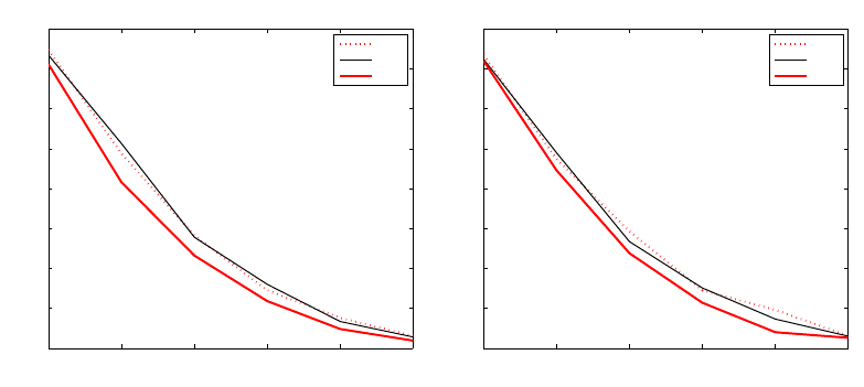
A KERNEL TWO-SAMPLE TEST

50 100 150 200 250 300

0.1

0.2

0.3

0.4

0.5

0.6

0.7

0.8

NEURO I, Bootstrap

Sample size m

Type II error

Train

Part

All

50 100 150 200 250 300

0.1

0.2

0.3

0.4

0.5

0.6

0.7

0.8

NEURO I, Pearson

Sample size m

Type II error

Train

Part

All

Figure 7: Type II error on the Neural Data I set, for kernel computed via the median heuristic on

the full data set (“All”), kernel computed via the median heuristic on a 10% hold-out

set (“Train”), and kernel computed via the median heuristic on 90% of the data (“Part”).

Results are plotted over 1000 repetitions. Left: Bootstrap results. Right: Pearson curve

results.

S. Andrews, I. Tsochantaridis, and T. Hofmann. Support vector machines for multiple-instance

learning. In Advances in Neural Information Processing Systems 15, Cambridge, MA, 2003.

MIT Press.

M. Arcones and E. Gin

e. On the bootstrap of u and v statistics. The Annals of Statistics, 20(2):

655–674, 1992.

F. R. Bach and M. I. Jordan. Kernel independent component analysis. Journal of Machine Learning

Research, 3:1–48, 2002.

P. L. Bartlett and S. Mendelson. Rademacher and Gaussian complexities: Risk bounds and structural

results. Journal of Machine Learning Research, 3:463–482, 2002.

S. Ben-David, J. Blitzer, K. Crammer, and F. Pereira. Analysis of representations for domain adap-

tation. In Advances in Neural Information Processing Systems 19, pages 137–144. MIT Press,

2007.

A. Berlinet and C. Thomas-Agnan. Reproducing Kernel Hilbert Spaces in Probability and Statistics.

Kluwer, 2004.

G. Biau and L. Gyorﬁ. On the asymptotic properties of a nonparametric l

-test statistic of homo-

geneity. IEEE Transactions on Information Theory, 51(11):3965–3973, 2005.

P. Bickel. A distribution free version of the Smirnov two sample test in the p-variate case. The

Annals of Mathematical Statistics, 40(1):1–23, 1969.

767

GRETTON, BORGWARDT, RASCH, SCH

OLKOPF AND SMOLA

C. L. Blake and C. J. Merz. UCI repository of machine learning databases, 1998. URL

http://www.ics.uci.edu/

∼

mlearn/MLRepository.html

K. M. Borgwardt, C. S. Ong, S. Schonauer, S. V. N. Vishwanathan, A. J. Smola, and H. P. Kriegel.

Protein function prediction via graph kernels. Bioinformatics (ISMB), 21(Suppl 1):i47–i56, Jun

2005.

K. M. Borgwardt, A. Gretton, M. J. Rasch, H.-P. Kriegel, B. Sch

olkopf, and A. J. Smola. Integrating

structured biological data by kernel maximum mean discrepancy. Bioinformatics (ISMB), 22(14):

e49–e57, 2006.

O. Bousquet, S. Boucheron, and G. Lugosi. Theory of classiﬁcation: a survey of recent advances.

ESAIM: Probability and Statistics, 9:323– 375, 2005.

R. Caruana and T. Joachims. KDD cup. 2004. URL

http://kodiak.cs.cornell.edu/kddcup/index.html

G. Casella and R. Berger. Statistical Inference. Duxbury, Paciﬁc Grove, CA, 2nd edition, 2002.

B. Chazelle. A minimum spanning tree algorithm with inverse-Ackermann type complexity. Journal

of the ACM, 47:1028–1047, 2000.

P. Comon. Independent component analysis, a new concept? Signal Processing, 36:287–314, 1994.

C. Cortes, M. Mohri, M. Riley, and A. Rostamizadeh. Sample selection bias correction theory. In

Proceedings of the International Conference on Algorithmic Learning Theory, volume 5254 of

Lecture Notes in Computer Science, pages 38–53. Springer, 2008.

M. Davy, A. Gretton, A. Doucet, and P. J. W. Rayner. Optimized support vector machines for

nonstationary signal classiﬁcation. IEEE Signal Processing Letters, 9(12):442–445, 2002.

V. de la Pe

na and E. Gin

e. Decoupling: from Dependence to Independence. Springer, New York,

1999.

M. Dud

ık and R. E. Schapire. Maximum entropy distribution estimation with generalized regu-

larization. In Proceedings of the Annual Conference on Computational Learning Theory, pages

123–138. Springer Verlag, 2006.

M. Dud

ık, S. Phillips, and R.E. Schapire. Performance guarantees for regularized maximum entropy

density estimation. In Proceedings of the Annual Conference on Computational Learning Theory,

pages 472–486. Springer Verlag, 2004.

R. M. Dudley. Real Analysis and Probability. Cambridge University Press, Cambridge, UK, 2002.

W. Feller. An Introduction to Probability Theory and its Applications. John Wiley and Sons, New

York, 2nd edition, 1971.

A. Feuerverger. A consistent test for bivariate dependence. International Statistical Review, 61(3):

419–433, 1993.

768

A KERNEL TWO-SAMPLE TEST

S. Fine and K. Scheinberg. Efﬁcient SVM training using low-rank kernel representations. Journal

of Machine Learning Research, 2:243–264, 2001.

R. Fortet and E. Mourier. Convergence de la r

eparation empirique vers la r

eparation th

eorique. Ann.

Scient.

Ecole Norm. Sup., 70:266–285, 1953.

J. Friedman. On multivariate goodness-of-ﬁt and two-sample testing. Technical Report SLAC-

PUB-10325, University of Stanford Statistics Department, 2003.

J. Friedman and L. Rafsky. Multivariate generalizations of the Wald-Wolfowitz and Smirnov two-

sample tests. The Annals of Statistics, 7(4):697–717, 1979.

K. Fukumizu, F. R. Bach, and M. I. Jordan. Dimensionality reduction for supervised learning with

reproducing kernel Hilbert spaces. Journal of Machine Learning Research, 5:73–99, 2004.

K. Fukumizu, A. Gretton, X. Sun, and B. Sch

olkopf. Kernel measures of conditional dependence. In

Advances in Neural Information Processing Systems 20, pages 489–496, Cambridge, MA, 2008.

MIT Press.

T. G

artner, P. A. Flach, A. Kowalczyk, and A. J. Smola. Multi-instance kernels. In Proceedings of

the International Conference on Machine Learning, pages 179–186. Morgan Kaufmann Publish-

ers Inc., 2002.

E. Gokcay and J.C. Principe. Information theoretic clustering. IEEE Transactions on Pattern Anal-

ysis and Machine Intelligence, 24(2):158–171, 2002.

A. Gretton, O. Bousquet, A.J. Smola, and B. Sch

olkopf. Measuring statistical dependence with

Hilbert-Schmidt norms. In Proceedings of the International Conference on Algorithmic Learning

Theory, pages 63–77. Springer-Verlag, 2005a.

A. Gretton, R. Herbrich, A. Smola, O. Bousquet, and B. Sch

olkopf. Kernel methods for measuring

independence. Journal of Machine Learning Research, 6:2075–2129, 2005b.

A. Gretton, K. Borgwardt, M. Rasch, B. Sch

olkopf, and A. Smola. A kernel method for the two-

sample problem. In Advances in Neural Information Processing Systems 15, pages 513–520,

Cambridge, MA, 2007a. MIT Press.

A. Gretton, K. Borgwardt, M. Rasch, B. Schlkopf, and A. Smola. A kernel approach to comparing

distributions. Proceedings of the 22nd Conference on Artiﬁcial Intelligence (AAAI-07), pages

1637–1641, 2007b.

A. Gretton, K. Borgwardt, M. Rasch, B. Sch

olkopf, and A. Smola. A kernel method for the two

sample problem. Technical Report 157, MPI for Biological Cybernetics, 2008a.

A. Gretton, K. Fukumizu, C.-H. Teo, L. Song, B. Sch

olkopf, and A. Smola. A kernel statistical

test of independence. In Advances in Neural Information Processing Systems 20, pages 585–592,

Cambridge, MA, 2008b. MIT Press.

A. Gretton, K. Fukumizu, Z. Harchaoui, and B. Sriperumbudur. A fast, consistent kernel two-sample

test. In Advances in Neural Information Processing Systems 22, Red Hook, NY, 2009. Curran

Associates Inc.

769

GRETTON, BORGWARDT, RASCH, SCH

OLKOPF AND SMOLA

G. R. Grimmet and D. R. Stirzaker. Probability and Random Processes. Oxford University Press,

Oxford, third edition, 2001.

P. Hall and N. Tajvidi. Permutation tests for equality of distributions in high-dimensional settings.

Biometrika, 89(2):359–374, 2002.

Z. Harchaoui, F. Bach, and E. Moulines. Testing for homogeneity with kernel Fisher discriminant

analysis. In Advances in Neural Information Processing Systems 20, pages 609–616. MIT Press,

Cambridge, MA, 2008.

M. Hein, T.N. Lal, and O. Bousquet. Hilbertian metrics on probability measures and their appli-

cation in SVMs. In Proceedings of the 26th DAGM Symposium, pages 270–277, Berlin, 2004.

Springer.

N. Henze and M. Penrose. On the multivariate runs test. The Annals of Statistics, 27(1):290–298,

1999.

W. Hoeffding. A class of statistics with asymptotically normal distribution. The Annals of Mathe-

matical Statistics, 19(3):293–325, 1948.

W. Hoeffding. Probability inequalities for sums of bounded random variables. Journal of the

American Statistical Association, 58:13–30, 1963.

T. Jebara and R. Kondor. Bhattacharyya and expected likelihood kernels. In Proceedings of the

Annual Conference on Computational Learning Theory, volume 2777 of LNCS, pages 57–71,

Heidelberg, Germany, 2003. Springer-Verlag.

N. L. Johnson, S. Kotz, and N. Balakrishnan. Continuous Univariate Distributions. Volume 1. John

Wiley and Sons, 2nd edition, 1994.

A. Kankainen. Consistent Testing of Total Independence Based on the Empirical Characteristic

Function. PhD thesis, University of Jyv

askyl

a, 1995.

D. Kifer, S. Ben-David, and J. Gehrke. Detecting change in data streams. In Proceedings of the

International Conference on Very Large Data Bases, pages 180–191. VLDB Endowment, 2004.

H.W. Kuhn. The Hungarian method for the assignment problem. Naval Research Logistics Quar-

terly, 2:83–97, 1955.

E. L. Lehmann and J. P. Romano. Testing Statistical Hypotheses. Springer, 3rd edition, 2005.

C. McDiarmid. On the method of bounded differences. In Survey in Combinatorics, pages 148–188.

Cambridge University Press, 1989.

C. Micchelli, Y. Xu, and H. Zhang. Universal kernels. Journal of Machine Learning Research, 7:

2651–2667, 2006.

A. M

uller. Integral probability metrics and their generating classes of functions. Advances in

Applied Probability, 29(2):429–443, 1997.

770

A KERNEL TWO-SAMPLE TEST

X.L. Nguyen, M. Wainwright, and M. Jordan. Estimating divergence functionals and the likelihood

ratio by penalized convex risk minimization. In Advances in Neural Information Processing

Systems 20, pages 1089–1096. MIT Press, Cambridge, MA, 2008.

W. H. Press, S. A. Teukolsky, W. T. Vetterling, and B. P. Flannery. Numerical Recipes in C. The Art

of Scientiﬁc Computation. Cambridge University Press, Cambridge, UK, 1994.

M. Rasch, A. Gretton, Y. Murayama, W. Maass, and N. K. Logothetis. Predicting spiking activity

from local ﬁeld potentials. Journal of Neurophysiology, 99:1461–1476, 2008.

M. Reed and B. Simon. Methods of modern mathematical physics. Vol. 1: Functional Analysis.

Academic Press, San Diego, 1980.

M. Reid and R. Williamson. Information, divergence and risk for binary experiments. Journal of

Machine Learning Research, 12:731–817, 2011.

P. Rosenbaum. An exact distribution-free test comparing two multivariate distributions based on

adjacency. Journal of the Royal Statistical Society B, 67(4):515–530, 2005.

Y. Rubner, C. Tomasi, and L.J. Guibas. The earth mover’s distance as a metric for image retrieval.

International Journal of Computer Vision, 40(2):99–121, 2000.

B. Sch

olkopf. Support Vector Learning. R. Oldenbourg Verlag, Munich, 1997. Download:

http://www.kernel-machines.org.

B. Sch

olkopf and A. Smola. Learning with Kernels. MIT Press, Cambridge, MA, 2002.

B. Sch

olkopf, J. Platt, J. Shawe-Taylor, A. J. Smola, and R. C. Williamson. Estimating the support

of a high-dimensional distribution. Neural Computation, 13(7):1443–1471, 2001.

B. Sch

olkopf, K. Tsuda, and J.-P. Vert. Kernel Methods in Computational Biology. MIT Press,

Cambridge, MA, 2004.

R. Serﬂing. Approximation Theorems of Mathematical Statistics. Wiley, New York, 1980.

J. Shawe-Taylor and N. Cristianini. Kernel Methods for Pattern Analysis. Cambridge University

Press, Cambridge, UK, 2004.

J. Shawe-Taylor and A. Dolia. A framework for probability density estimation. In Proceedings of

the International Conference on Artiﬁcial Intelligence and Statistics, pages 468–475, 2007.

H. Shen, S. Jegelka, and A. Gretton. Fast kernel-based independent component analysis. IEEE

Transactions on Signal Processing, 57:3498 – 3511, 2009.

B. W. Silverman. Density Estimation for Statistical and Data Analysis. Monographs on statistics

and applied probability. Chapman and Hall, London, 1986.

N.V. Smirnov. On the estimation of the discrepancy between empirical curves of distribution for

two independent samples. Moscow University Mathematics Bulletin, 2:3–26, 1939. University

of Moscow.

771

GRETTON, BORGWARDT, RASCH, SCH

OLKOPF AND SMOLA

A. J. Smola and B. Sch

olkopf. Sparse greedy matrix approximation for machine learning. In Pro-

ceedings of the International Conference on Machine Learning, pages 911–918, San Francisco,

2000. Morgan Kaufmann Publishers.

A. J. Smola, A. Gretton, L. Song, and B. Sch

olkopf. A Hilbert space embedding for distributions.

In Proceedings of the International Conference on Algorithmic Learning Theory, volume 4754,

pages 13–31. Springer, 2007.

L. Song, X. Zhang, A. Smola, A. Gretton, and B. Sch

olkopf. Tailoring density estimation via re-

producing kernel moment matching. In Proceedings of the International Conference on Machine

Learning, pages 992–999. ACM, 2008.

B. Sriperumbudur, A. Gretton, K. Fukumizu, G. Lanckriet, and B. Sch

olkopf. Injective Hilbert space

embeddings of probability measures. In Proceedings of the Annual Conference on Computational

Learning Theory, pages 111–122, 2008.

B. Sriperumbudur, K. Fukumizu, A. Gretton, G. Lanckriet, and B. Schoelkopf. Kernel choice

and classiﬁability for RKHS embeddings of probability distributions. In Advances in Neural

Information Processing Systems 22, Red Hook, NY, 2009. Curran Associates Inc.

B. Sriperumbudur, K. Fukumizu, A. Gretton, B. Sch

olkopf, and G. Lanckriet. Non-parametric

estimation of integral probability metrics. In International Symposium on Information Theory,

pages 1428 – 1432, 2010a.

B. Sriperumbudur, A. Gretton, K. Fukumizu, G. Lanckriet, and B. Sch

olkopf. Hilbert space em-

beddings and metrics on probability measures. Journal of Machine Learning Research, 11:1517–

1561, 2010b.

B. Sriperumbudur, K. Fukumizu, and G. Lanckriet. Universality, characteristic kernels and RKHS

embedding of measures. Journal of Machine Learning Research, 12:2389–2410, 2011a.

B. Sriperumbudur, K. Fukumizu, and G. Lanckriet. Learning in Hilbert vs. Banach spaces: A mea-

sure embedding viewpoint. In Advances in Neural Information Processing Systems 24. Curran

Associates Inc., Red Hook, NY, 2011b.

I. Steinwart. On the inﬂuence of the kernel on the consistency of support vector machines. Journal

of Machine Learning Research, 2:67–93, 2001.

I. Steinwart and A. Christmann. Support Vector Machines. Information Science and Statistics.

Springer, 2008.

I. Takeuchi, Q. V. Le, T. Sears, and A. J. Smola. Nonparametric quantile estimation. Journal of

Machine Learning Research, 7, 2006.

D. M. J. Tax and R. P. W. Duin. Data domain description by support vectors. In Proceedings

ESANN, pages 251–256, Brussels, 1999. D Facto.

A. W. van der Vaart and J. A. Wellner. Weak Convergence and Empirical Processes. Springer, 1996.

L. Wasserman. All of Nonparametric Statistics. Springer, 2006.

772

A KERNEL TWO-SAMPLE TEST

J. E. Wilkins. A note on skewness and kurtosis. The Annals of Mathematical Statistics, 15(3):

333–335, 1944.

C. K. I. Williams and M. Seeger. Using the Nystrom method to speed up kernel machines. In

Advances in Neural Information Processing Systems 13, pages 682–688, Cambridge, MA, 2001.

MIT Press.

773